Response outcome gates the effect of spontaneous cortical state fluctuations on perceptual decisions
- Champalimaud Research, Champalimaud Foundation, Portugal
Figures
Figure 1 with 1 supplement
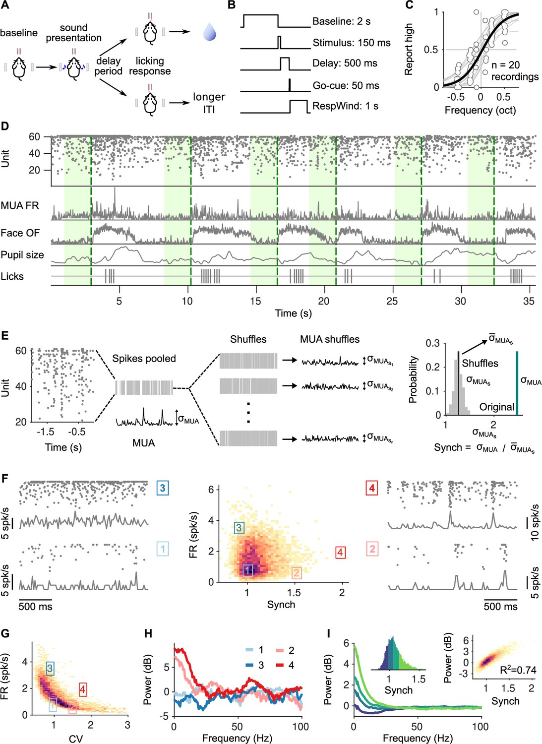
Task structure, signals monitored, and quantification of synchrony in baseline activity.
(A) Task schematic. Head-fixed mice lick at one of two spouts depending on whether the frequency of a pure tone is higher or lower than 14 kHz. (B) Temporal sequence of events in a trial. Mice should respond after a delay of 0.5 s. Baseline activity is analyzed in a window of 2 s before the presentation of the sound. (C) Discrimination performance. Each dot is the proportion of times a mouse reports high in a given recording session to a given sound. Solid curve is a logistic regression fit. (D) Signals monitored. Top to bottom are population raster, multiunit firing rate (MUA FR), mean optic flow of the face (OpticF), size of the pupil (PupilS), and licks. Dashed vertical lines mark stimulus presentation times and green background marks the baseline period we analyze. (E) Method for quantifying synchronization. Synch effectively measures the population averaged correlation in the baseline period relative to surrogate data with the same number of spikes but randomly placed in the same period of time (Methods). (F) Distribution of baseline FR and Synch pooled across all recording sessions. Plots on the sides show rasters and population firing rates for four example baseline periods. (G) Identical plot to the one in (F)-middle, but where global synchronization is assessed using the coefficient of variation (CV) of the instantaneous population rate (Methods). CV and FR are negatively correlated. (H) Power spectrum (Methods) of the four individual example baseline periods in (F). (I) Average power spectrum of each of the four quantiles of the distribution of Synch across trials. Large values of Synch reflect low-frequency coordinated fluctuations across the population. Inset left: Aggregate distribution of Synch values across recordings. Each quantile corresponds to one of the spectra in panel (I). Inset right: Relationship between Synch and average MUA power in the 4–16 Hz range.
Figure 1—figure supplement 1
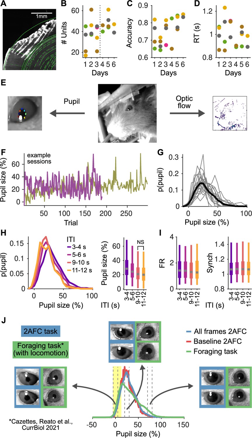
Histology, stability of the recordings and behavior over multiple sessions and pupil size analyses.
(A) Reconstruction of a brain slice with the shanks of the probe marked with DiI. Shank tips in this recording were in the primary auditory cortex (areas adapted from the Paxinos and Franklin, 2007). (B) Number of units recorded in each session. Each color represents a mouse. (C) Accuracy for each mouse as a function of the recording session. (D) Median reaction time of each animal as a function of the recording session. (E) Middle: Image of the face of the mouse in our setup. Left: From these videos we extract pupil size using DeepLabCut (Mathis et al., 2018), marking eight points to characterize the ellipse for each pupil. Right: From the same videos we also compute the optic flow – to quantify facial movement – by computing the average difference in pixel intensity across adjacent frames (in color in the figure). (F) Example of pupil size in the pre-stimulus period in two example sessions. In both sessions, pupil size fluctuates strongly on a trial by trial basis. In one session, there is also a general trend for an increase in pupil size throughout the session. (G) Distribution of pupil size. Each line represents a session and the black line indicates the distribution of the pooled data. 0% indicate the minimum pupil size (Methods) and so 100% indicates trials were pupil size was double relative to the minimum. (H) Left: Distribution of pupil size as a function of the inter-trial interval (ITI). Right: Whisker plots (2.5th, 25th, 50th, 75th, and 97.5th quantiles) for the distributions of pupil size. Median pupil sizes are approximately 10% larger (relative to the minimum), and more variable for the shortest ITIs and decay to a steady state by approximately 10 s. The distributions for all ITI ranges largely overlap and all have significant mass at contracted pupil sizes smaller than 20%. (I) Same as (H, right) but for the distributions of baseline firing rate (FR; middle) and Synch (right) as a function of the ITI. Distributions of FR and Synch are essentially independent of the ITI. (J) Comparison of pupil size distributions between our task (both all video frames [blue] or just during the two second baseline [red]) and a foraging task (green; Cazettes et al., 2021) where mice run in a treadmill and trials are self-paced. Blue and red distributions are almost completely overlapping, indicating that the range of pupil size in the baseline period represents well the distribution in the session. The green distribution has more mass at large pupil sizes, corresponding to periods of locomotion and sustained licking. The region in yellow marks the range of contracted pupil sizes, where the distributions in both tasks are highly overlapping. Insets show example frames from contracted (sizes [−5,5]%), intermediate ([20,30]%), and dilated ([70,80]%) pupils (indicated by vertical dashed lines). Slightly larger pupil sizes in our task reflect the different lighting conditions in the two experiments: in our experiment, the task took place in a sound isolation box with restricted light, whereas in Cazettes et al., 2021, the task took place in an open Faraday cage, with ambient light and a strip of LEDs turned on and visible to the mice during the whole behavioral session.
Figure 2 with 2 supplements
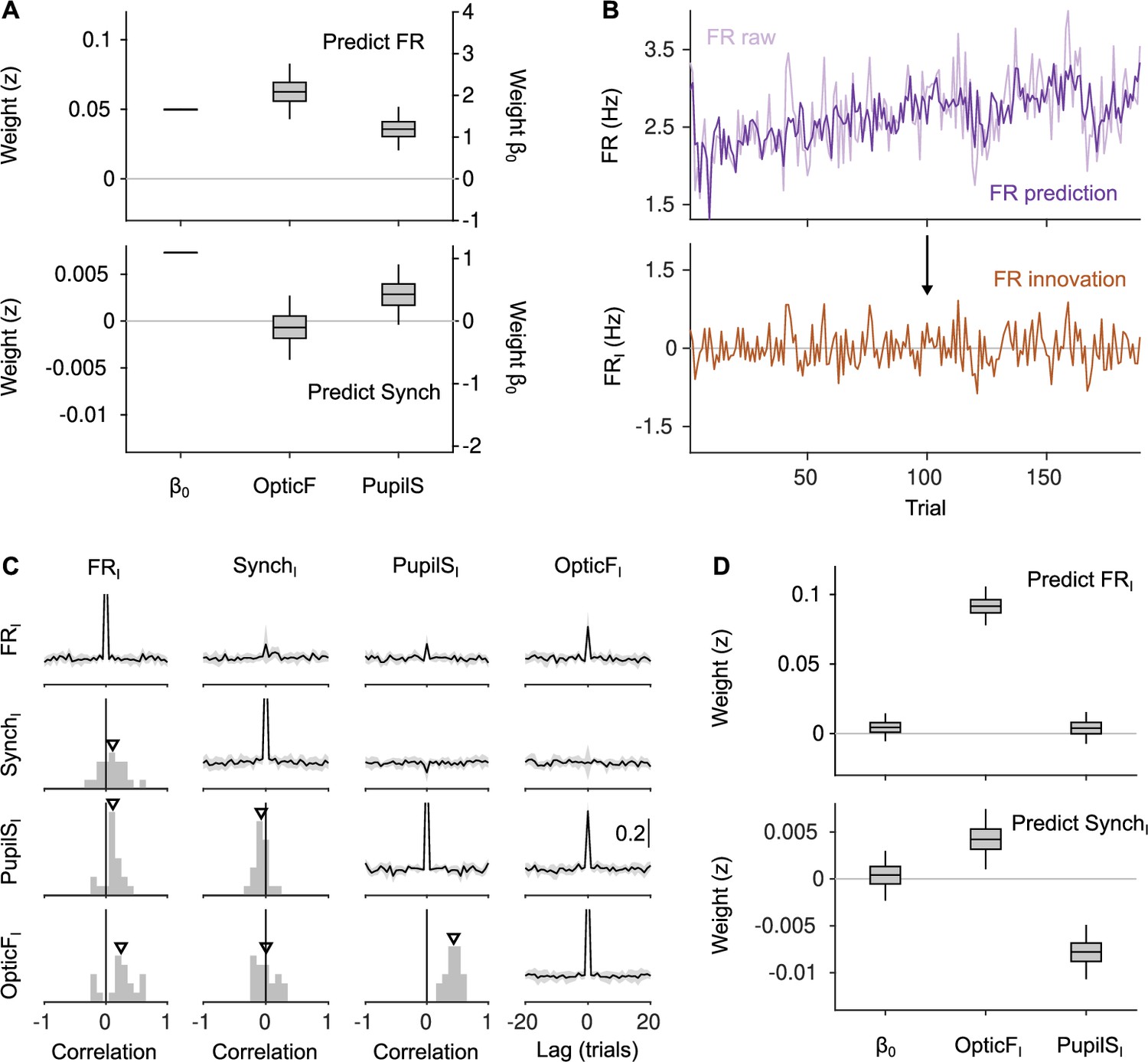
Innovations clarify the effect of movement and pupil size on cortical state fluctuations.
(A) Linear mixed model regression (Methods) of firing rate (FR; top) and Synch (bottom) on movement and pupil size. Graphs show values of regression coefficients. Box plots here and elsewhere represent median, interquartile range and 95% confidence interval (CI) on the bootstrap distribution of the corresponding parameter (Methods). Offset can be read from the right y-axis. (B) Example of the process of calculating innovations for the baseline FR of one recording session. Top, raw data and prediction of the raw data (Figure 2—figure supplement 2; Methods). The innovation FRI (bottom) is the difference (prediction residual) between the two traces in the top. (C) Correlation between OpticF, PupilS, FR, and Synch innovations. Diagonal and above, cross-correlations between each of the four signals (black, median across recordings; gray, median absolute deviation [MAD]). Below diagonal. For each pair of innovations, histogram across recordings of their instantaneous correlation. Triangles mark the median across recordings. (D) Identical analysis as panel (A) but using innovations instead of the raw signals.
Figure 2—figure supplement 1
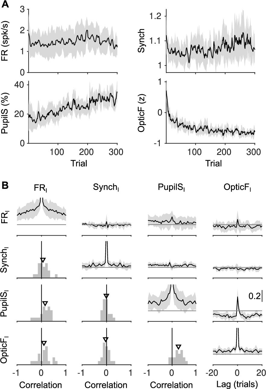
Slow trends of baseline signals during the session.
(A) Median (black) and median absolute deviation (MAD; gray shading) across sessions of each of the four baseline signals. All the signals display slow trends and in some cases monotonic increases or decreases through the recording session. (B) Diagonal and above shows the auto- and cross-correlations of each of the four baseline signals (median ± MAD). Below diagonal shows the histogram of the instantaneous correlation between each pair of signals across sessions. Triangle is the median across sessions (same format as Figure 2C). Non-zero values of auto- and cross-correlations far from zero lag reflect existence of slow timescales, which are eliminated by our cross-whitening procedure (Methods, Figure 2—figure supplement 2) and are thus absent from the equivalent analysis performed on innovations (Figure 2 in the main text.).
Figure 2—figure supplement 2

Constructing innovations by cross-whitening.
(A) Schematic description of the linear fit and associated residuals used to generate the firing rate (FR) innovations. The same procedure was used for Synch, PupilS, and OpticF. (B) Example traces for obtaining the PupilS innovations in one recording. Left, raw and linear fit of the PupilS. Right, residuals. (C) Histogram across sessions of the fraction of variance () explained by the linear fits of each of the four signals. Triangle is the median of each histogram.
Figure 3 with 6 supplements
The effect of spontaneous state fluctuations on accuracy is outcome dependent.
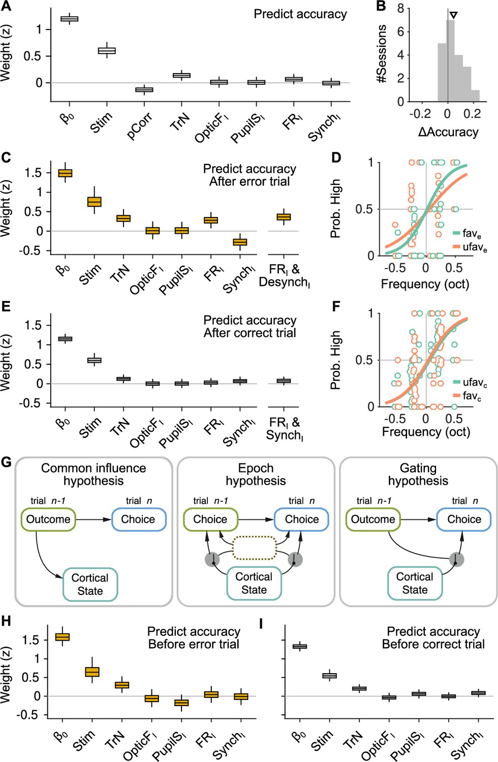
(A) Coefficients of a generalized linear mixed model (GLMM) fit to the mice’s choice accuracy in valid trials. Accuracy is affected by the strength of evidence, the point during the session and the outcome of the previous trial, but none of the four signals computed during the baseline explain accuracy. (B) Mean difference in accuracy after errors minus after corrects in each of the recording sessions. Triangle, median across sessions. (C) GLMM fit to accuracy computed separately after error trials. On the right, we show the distribution of a single coefficient capturing trial-to-trial fluctuations in desynchronization and firing rate simultaneously (see text). (D) Psychometric function (logistic fit, Methods) of aggregate data across sessions separately for trials with favorable ( and ) and unfavorable ( and ) baseline states after a error trials. (E, F) Same as (C, D) but for choices after a correct trial. Note that, based on the results in (E), the favorable state after a correct trial is and . (G) Schematic illustration of possible relationships between outcome, baseline cortical state and accuracy. Left, the association between state and accuracy is spurious and results from a common effect of response outcome on these two variables. Middle, epoch hypothesis (see text). An unmeasured variable with a timescale of several trials mediates both the effect of state on accuracy and the prevalence of errors. Right, response outcome gates the effect of state fluctuations (errors open the gate) on choice accuracy. (H, I) Same as (C, E) but conditioned on the outcome of the next, rather than the previous trial.
Figure 3—figure supplement 1

Robustness of the association between brain state and accuracy.
(A) Parametric estimation of confidence intervals (CIs) for accuracy fits. Equivalent to Figure 3C, E, but circle and bars show the mean and 95% CI for each coefficient reported by fitglme (Methods) using an approximation to the conditional mean squared error of prediction (CMSEP) method (Booth and Hobert, 1998). (B) Generalized linear mixed model (GLMM) analysis designed to separately test the effect of cortical state on discriminability () and bias (criterion). To do this, we predict the animal’s choice on each trial, not whether the outcome of the trial was correct (as in Figure 3C, E). We used the combined FRI–SynchI predictor which captures, as a single scalar, how favorable the cortical state is for accuracy after errors or correct trials. Considering this predictor as a main effect can capture the effect of cortical state on bias, whereas the interaction between this predictor and the stimulus strength can capture an effect of cortical state on discriminability. Cortical state is only predictive of choice as an interaction term after errors (p = 0.0025). Error bars are computed using parametric estimation. (C) GLMM fit to accuracy computed separately after error trials (left) and correct trials (right) considering recording session as a random effect nested within mouse. Error bars are computed using parametric estimation.
Figure 3—figure supplement 2
Generalized linear mixed model (GLMM) analysis including quadratic terms and differentially for superficial and deep recording shanks.
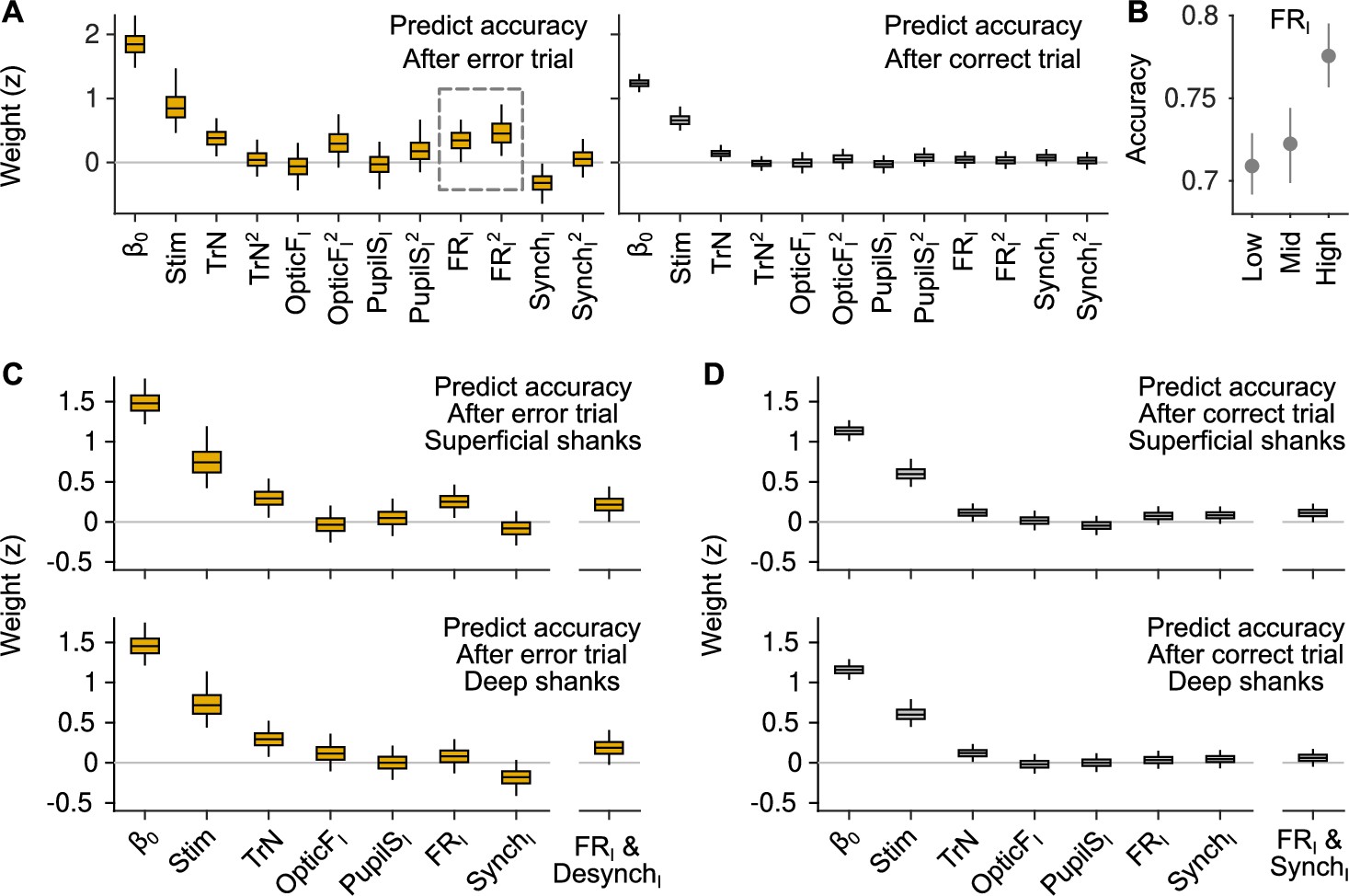
(A) GLMM fit to accuracy for trials following errors (left) and correct responses (right). Differently from the GLMMs in Figure 3, this model includes quadratic terms for TrN, OpticFI, PupilSI, FRI, and SynchI. The only significant quadratic term is the one for FRI after errors. (B) Accuracy as a function of FRI after error trials. The relationship between FRI and accuracy is supralinear and resembles a quadratic function (median and 50% confidence interval [CI] derived using bootstrap), as suggested by the results of the GLMM in (A). (C) GLMM fit to accuracy after error trials using FRI and SynchI predictors that were built using (putative) superficial or deep neurons in the recordings. (D) Same analysis as in (C) but considering only trials after correct responses.
Figure 3—figure supplement 3

Robustness of the results on the effects of cortical state on accuracy.
(A) The analysis in Figure 3C–E was repeated but shifting the window 2 s into the past (i.e., window is centered 3 s before stimulus onset, instead of 1 s as in the manuscript). Although the full model was fitted, we only display the magnitude of the firing rate and synchrony innovation predictors. (B) Same but changing the window duration. For the three cases on the right (for each outcome), the center of the window is still at 1 s before the stimulus, as in the manuscript. The first case shows the results for a window [−4 0] s. Overall, these results show that if the window is either too short, or if it moves away too much from the presentation of the sound, the predictive power of baseline activity innovations after errors wanes. However, this (expected) degradation is gradual. Innovations of baseline fluctuations are never predictive of accuracy after correct trials, independently of the window used for measuring baseline activity.
Figure 3—figure supplement 4

Lack of association between slow cortical state fluctuations and accuracy.
(A) For an example session, we show the raw firing rate (FR; top), Synch (middle top) during the baseline and accuracy (middle bottom) in that trial. Bottom: We smoothed each of these signals with a running window of 10 trials, removed the session-wide linear trend, and z-scored. (B) Left: Cross-correlation function between the smoothed accuracy and FR time series. Each gray line is a recording and the black line is the mean. Right: Histogram across recordings of the cross-correlation function at zero lag. (C) Same as (B) but for the cross-correlation between the smoothed accuracy and Synch time series.
Figure 3—figure supplement 5
Behavioral predictions including slow trends.
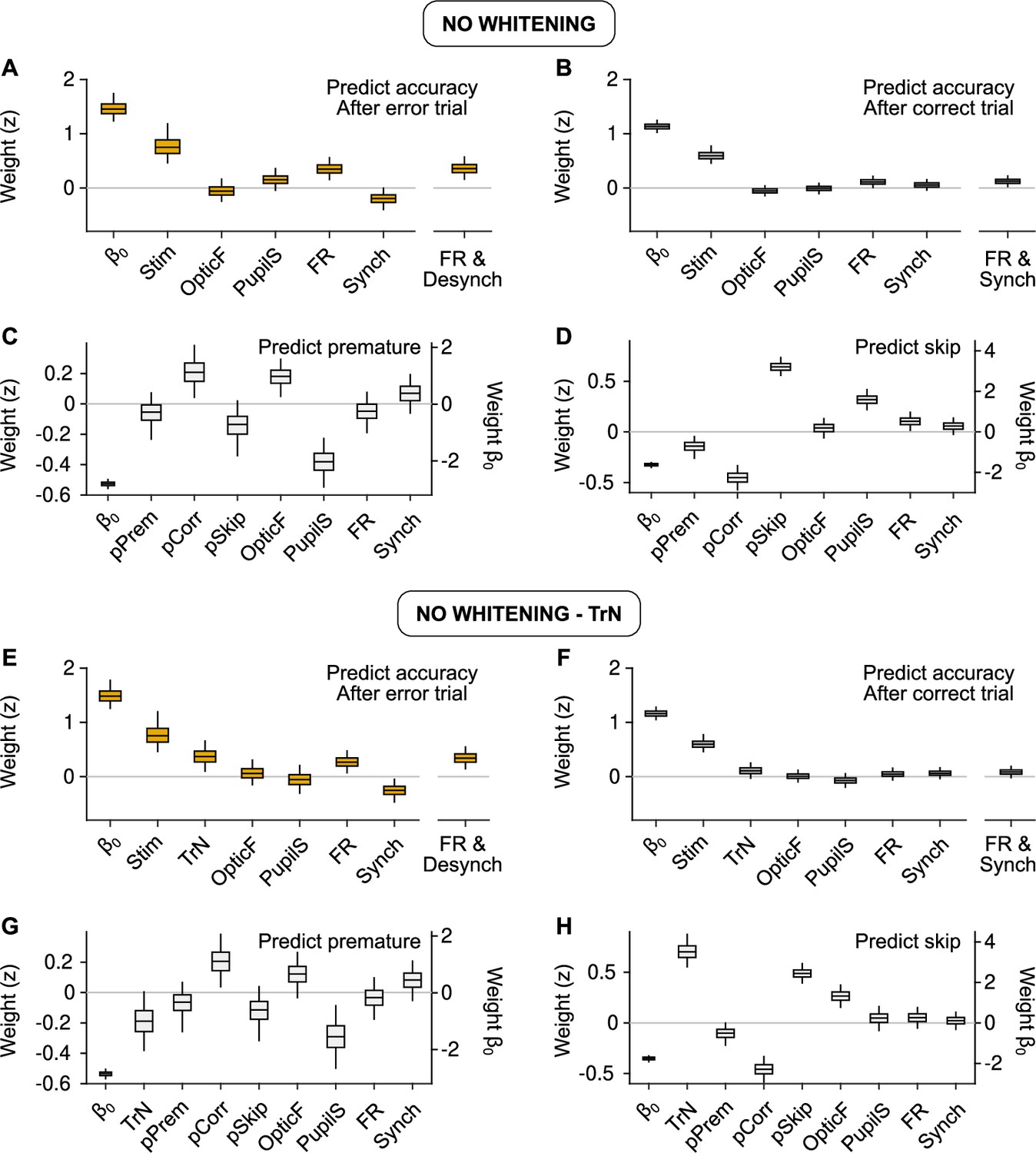
(A, E) Equivalent to Figure 3C (predicting accuracy after errors) but using raw predictors without (A) or with (E) the session trend TrN. (B, F) Same, but equivalent to Figure 3E (predicting accuracy after correct trials). (C, G) Same, but equivalent to Figure 5D (predicting premature trials). (D, H) Same, but equivalent to Figure 5F (predicting Skips). These results are largely equivalent to the ones in the main text using innovations, suggesting that, on average across recordings, slow trends in the baseline signals are not associated in a reliable fashion to accuracy, or the probabilities of premature responding or Skips. If the session trend regressor TrN is not included, the fit to Skips changes, revealing a spurious relationship between Pupil size and Skip probability that arises exclusively by the common increase in both of these variables throughout the session.
Figure 3—figure supplement 6
Outcome dependence of the effect of cortical state on stimulus and choice discriminability from evoked responses.
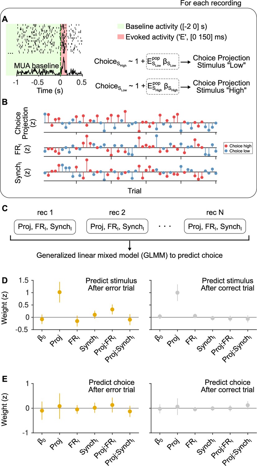
(A) Schematic of our approach. We calculated evoked firing rates in each trial for each neuron in a window of [0 150] ms starting at sound stimulus onset. FRI and SynchI predictors during the [−2 0] s baseline period were the same as in the text. When examining choice discriminability, for each experiment we computed a ‘choice axis’ separately for each of the two stimulus categories using cross-validated regularized logistic regression (see Methods). (B) Using this axis, we computed a scalar ‘choice projection’ for each trial which, together with the baseline regressors FRI and SynchI, constituted the data from each experiment in this analysis. (C) We then aggregated these data from all experiments in a generalized linear mixed model (GLMM) in order to predict choice trial-by-trial, using ‘recording session’ as a random effect. The same exact procedure was used to examine stimulus category discriminability, computing a ‘stimulus axis’ separately for each choice in each recording. (D) Magnitude of the coefficients for each regressor in a GLMM used to predict stimulus category after error (left) and after correct (right) trials. After errors, the interaction between the stimulus projection and FRI is positive and significant ( = 0.002; 95% confidence interval [CI] = [0.12,0.52]) and the median of the interaction between the stimulus projection and SynchI is negative, but not significant ( = 0.40; 95% CI = [−0.32,0.13]). After correct trials, none of the interactions are significant. (E) Same but for choice predictions. Regardless of outcome, the magnitude of the coefficient for the choice projection is not significant, signaling that we cannot detect a non-zero choice probability in our dataset. As expected given the lack of a main effect for the choice projection, the interaction terms with FRI and SynchI are also not significantly different from zero, although the median of the coefficients for each outcome is consistent with the expectation given the results in Figure 3.
Figure 4
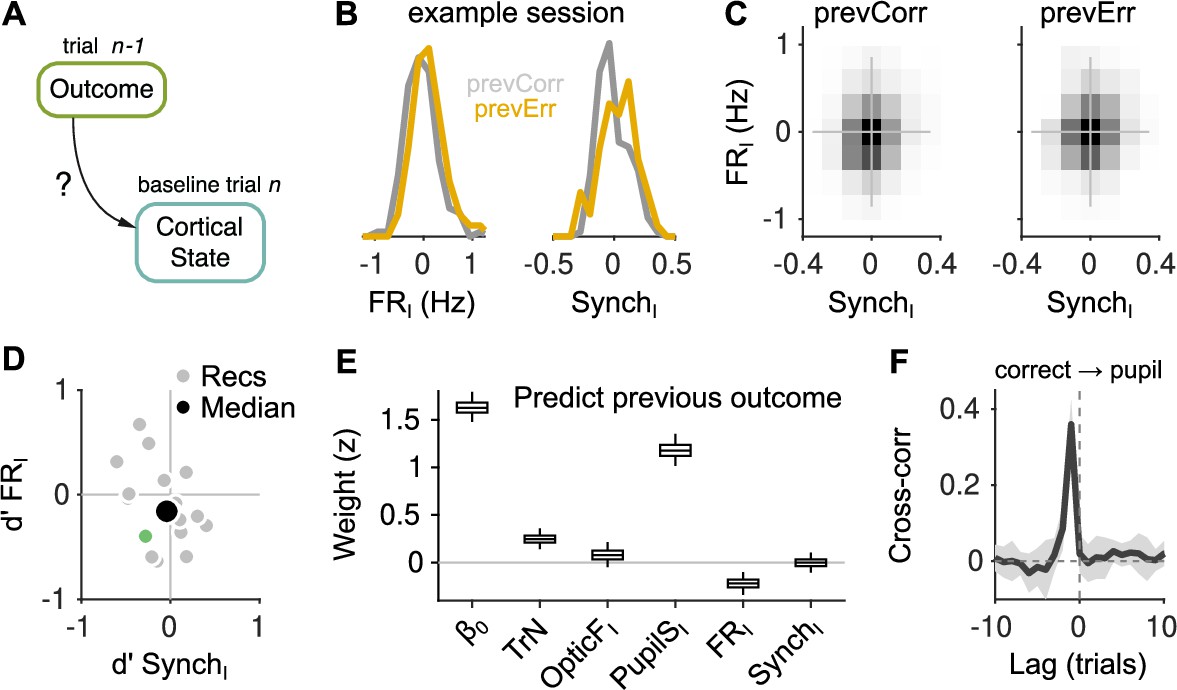
Effect of outcome on baseline activity.
(A) Schematic illustration of the question addressed in this figure. (B) Distribution of FRI (left) and SynchI (right) after each of the two outcomes for an example session. (C) Joint histogram of FRI and SynchI on aggregate across recordings after a correct (left) and after an error (right) trial. (D) Discriminability index between the distributions of FRI and SynchI (such as those in (B)) after each of the two outcomes. Each gray dot corresponds to one recording, the colored dot is the example recording in (B), and the large black circle is the median. (E) Coefficients of a generalized linear mixed model (GLMM) fit to the outcome (correct or error) of the mice’s choices on trial using as regressors TrN and innovations from the baseline of trial . (F) Cross-correlation function between the raw outcome and PupilS time series (Methods). Black is the median across recordings, gray is the median absolute deviation (MAD). Throughout this figure, innovations were modified so as to exclude previous outcomes in the calculations of the residuals (Methods).
Figure 5 with 1 supplement
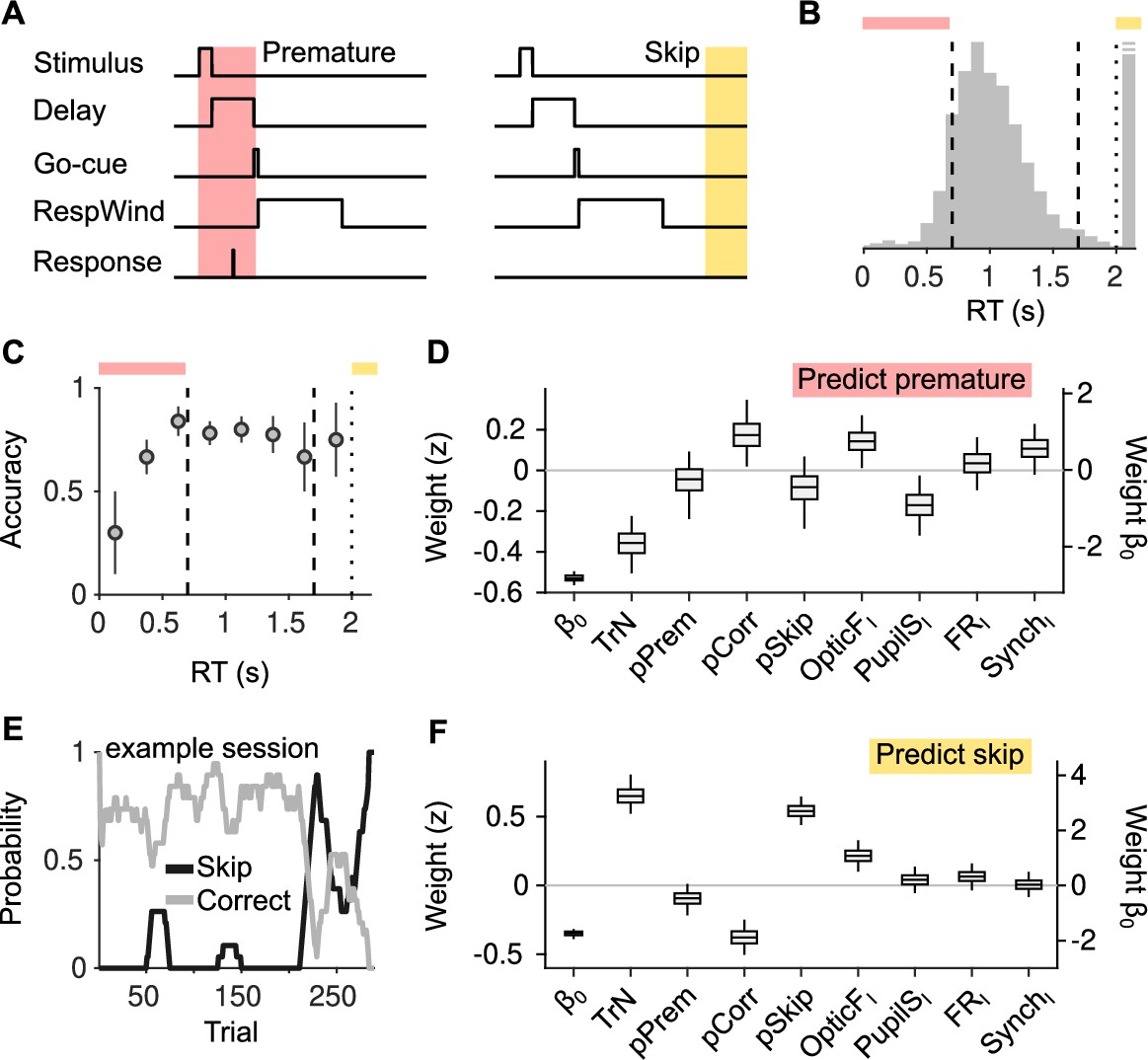
Effect of cortical state fluctuations on premature responding and engagement.
(A) Definition of premature responses and skips. (B) Aggregate across sessions of the distribution of reaction times (RTs) in our task. Dashed lines indicate the response window in which a correct response was rewarded (valid trials). Trials where a response is not produced before the dotted line are defined as skips. Top, colors used to signal each trial type in (B). (C) Accuracy (median ± median absolute deviation [MAD] across recordings) conditional on RT. (D) Coefficients of a generalized linear mixed model (GLMM) fit to explain whether a given trial is premature or valid. Magnitude of the offset () should be read of from the right y-axis. (E) Probability of not responding to the stimulus (skip) in an example session. Skips tend to occur in bouts and are more frequent toward the end of the session. (F) Same as (D) but for a GLMM aimed at explaining if a particular trial is a skip or valid.
Figure 5—figure supplement 1
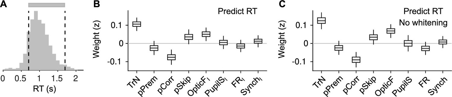
Explaining reaction time (RT) in valid trials.
(A) Histogram of RTs (equivalent to Figure 5A). For this figure, we attempt to explain RTs within the two dashed lines (gray bar), that is, during valid trials. (B) Coefficients of a LMM explaining RT using the same predictors as in our other analyses on responsivity in Figure 5D, F. Coefficients for session trend and previous outcome are positive and negative, respectively ( and , bootstrap), showing that mice tend to slow down through the session – consistent with them progressively losing motivation – and also after an error – revealing that post-error slowing down is evident despite the delay period in the task. Although the pSkip coefficient is not significant (, bootstrap), mice tend to be slower in responding after a disengaged trial, suggesting a continuity between long RTs and lack of response. This is consistent with the positive association between facial movement in the baseline (OpticFI) and RT (, bootstrap), which is also present in the prediction of skips (Figure 5F). Neither pupil size, firing rate, or synchrony innovations explain RT (, , and for PupilSI, FRI, and SynchI, respectively, bootstrap). (C) Same as (B) but without cross-whitening the predictors.
Author response image 1
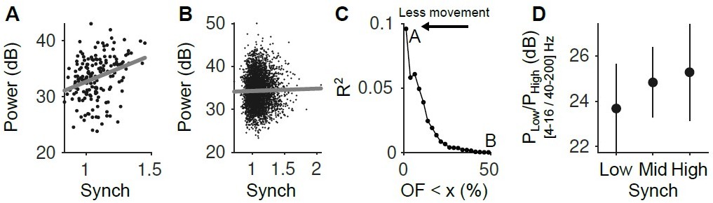
(A) Relationship between the LFP power (4-16 Hz) and the Synch measurement used to estimate the synchrony of the neuronal population in the pre-stimulus periods ([-2 0] s). Only the trials with the smallest facial movements were considered (2.5% of the trials with the lowest OpticF values). (B) Same as A but considering the 50% trials with the smaller movement. (C) R2 of the regression of LFP power in the 4-16 Hz range on our Synch measure as a function of the percentile of trials used from the baseline facial movement distribution. The more movement, the more the relationship between the LFP and Synch is obscured. (D) Power ratio between low (4-16 Hz) and high (40-200 Hz) frequency components of the LFP as a function of neural synchrony (for the fraction of trials in the lowest 2.5 percentile of baseline OpticF).
Additional files
-
Supplementary file 1
We report in a table the statistics associated to the fixed coefficients in each of the generalized linear mixed models described in the main text.
Starting from the left, each column represents: the figure in the text where the results are displayed, the prediction target, the predictors (one row per predictor), the median and lower and upper limits of the 95% confidence interval (Methods), the associated bootstrap p value (Methods), and the total number of observations (number of rows in the predictor matrix) in the model.
- https://cdn.elifesciences.org/articles/81774/elife-81774-supp1-v3.pdf
-
MDAR checklist
- https://cdn.elifesciences.org/articles/81774/elife-81774-mdarchecklist1-v3.docx
Download links
A two-part list of links to download the article, or parts of the article, in various formats.
Downloads (link to download the article as PDF)
Open citations (links to open the citations from this article in various online reference manager services)
Cite this article (links to download the citations from this article in formats compatible with various reference manager tools)
Response outcome gates the effect of spontaneous cortical state fluctuations on perceptual decisions
eLife 12:e81774.
https://doi.org/10.7554/eLife.81774


