Research Article

Neuroscience

Network instability dynamics drive a transient bursting period in the developing hippocampus in vivo

Department of Neurology, Jena University Hospital, Germany
Section Translational Neuroimmunology, Jena University Hospital, Germany
Department of Psychology, Technical University Dresden, Germany
Department of Neurophysiology, Institute of Physiology, University of Würzburg, Germany

Dec 19, 2022

https://doi.org/10.7554/eLife.82756

Version of Record

Accepted for publication after peer review and revision.

Download
Cite
Share
CommentOpen annotations (there are currently 0 annotations on this page).

450 views

Version of Record published: December 19, 2022 (This version)
Accepted: December 5, 2022
Received: August 16, 2022
Preprint posted: May 29, 2021 (Go to version)

1. Of interest
Early-life experience reorganizes neuromodulatory regulation of stage-specific behavioral responses and individuality dimensions during development

Reemy Ali Nasser, Yuval Harel, Shay Stern

Research Article Updated Jun 1, 2023
Further reading

Article
Figures and data
Abstract
Editor's evaluation
Introduction
Results
Discussion
Methods
Appendix 1
Data availability
References
Decision letter
Author response
Article and author information
Metrics

Abstract

Spontaneous correlated activity is a universal hallmark of immature neural circuits. However, the cellular dynamics and intrinsic mechanisms underlying network burstiness in the intact developing brain are largely unknown. Here, we use two-photon Ca²⁺ imaging to comprehensively map the developmental trajectories of spontaneous network activity in the hippocampal area CA1 of mice in vivo. We unexpectedly find that network burstiness peaks after the developmental emergence of effective synaptic inhibition in the second postnatal week. We demonstrate that the enhanced network burstiness reflects an increased functional coupling of individual neurons to local population activity. However, pairwise neuronal correlations are low, and network bursts (NBs) recruit CA1 pyramidal cells in a virtually random manner. Using a dynamic systems modeling approach, we reconcile these experimental findings and identify network bi-stability as a potential regime underlying network burstiness at this age. Our analyses reveal an important role of synaptic input characteristics and network instability dynamics for NB generation. Collectively, our data suggest a mechanism, whereby developing CA1 performs extensive input-discrimination learning prior to the onset of environmental exploration.

Editor's evaluation

This study provides fundamental findings about the developing brain and compelling evidence for how hippocampal physiology evolves during the first few postnatal weeks. Unlike previous in vitro results, which find declining network synchrony after the first postnatal week, the authors find in vivo that synchrony increases and peaks in the second postnatal week, despite emerging GABA-mediated inhibition during this time. They develop a model to explain these findings and suggest an underlying bistable population dynamic, oscillating between silent and active states, that sculpts input discrimination and network synchrony.

https://doi.org/10.7554/eLife.82756.sa0

Introduction

Developing neural circuits generate correlated spontaneous activity in which co-activations of large groups of neurons are interspersed by relatively long periods of quiescence (Kirmse and Zhang, 2022; Molnár et al., 2020). In rodents, network activity commences long before the onset of hearing, vision, and active environmental exploration and makes important contributions to the proper assembly of brain circuits (Kirkby et al., 2013). Activity-dependent refinements operate at multiple steps of maturation, including the control of neural progenitor progression (Vitali et al., 2018), apoptotic cell death (Blanquie et al., 2017; Wong et al., 2018), neuronal cell-type specification (Sun et al., 2018), migration (Maset et al., 2021) as well as synapse formation and plasticity (Oh et al., 2016; Sando et al., 2017; Winnubst et al., 2015). Experimental and theoretical evidence suggest that, in addition to the overall level of activity, specific spatiotemporal firing patterns are critical for activity-dependent refinements to occur (Albert et al., 2008; Zhang et al., 2011).

A representative example of correlated spontaneous network activity is found in the neonatal hippocampus in vivo. During the first postnatal week, the main electrophysiological signature is bursts of multi-unit activity (Leinekugel et al., 2002), which bilaterally synchronize large parts of the dorsal CA1 and are often accompanied by sharp waves (SPWs) in the local field potential (Valeeva et al., 2019; Valeeva et al., 2020). SPWs frequently follow myoclonic limb or whisker twitches (Dard et al., 2022; Del Rio-Bermudez et al., 2020; Karlsson et al., 2006; Valeeva et al., 2019), suggesting that SPWs convey feedback information from the somatosensory periphery. By the second postnatal week, discontinuous activity in the olfactory bulb drives network oscillations in the entorhinal cortex (Gretenkord et al., 2019), further pointing to a role of multi-sensory integration in limbic ontogenesis. In the neonatal CA1, recent in vivo investigations revealed that GABAergic interneurons (INs) could promote a second class of SPW-independent network events through NKCC1-dependent chloride uptake in pyramidal cells (PCs), although inhibitory effects of GABAergic signaling coexist (Graf et al., 2021; Murata and Colonnese, 2020; but see Valeeva et al., 2016). A qualitatively similar situation applies to the immature hippocampus in vitro (Ben-Ari et al., 1989; Flossmann et al., 2019), in which correlated spiking of PCs is facilitated by increasing the intracellular chloride concentration (Spoljaric et al., 2019; Zhang et al., 2019), whereas inhibition of chloride uptake has the opposite effect (Dzhala et al., 2005). In this line, in vitro studies suggest that correlated spontaneous activity largely disappears by the beginning of the second postnatal week, when the reversal potential of GABA_A receptor-mediated currents shifts into the hyperpolarizing direction (Spoljaric et al., 2017; Tyzio et al., 2008). However, the developmental trajectories of cellular network firing dynamics in the hippocampus in vivo remain largely unknown.

Using two-photon Ca²⁺ imaging, we here provide a detailed analysis of the spatiotemporal dynamics of network activity in the developing CA1 region at single-cellular resolution in vivo. We reveal that CA1 PCs undergo a transient period of enhanced burst-like network activity during the second postnatal week, when GABA already acts as an inhibitory transmitter. Our results show that, at this time, network bursts (NBs) recruit CA1 PCs in an almost random manner, and recurring cellular activation patterns become more stable only after eye opening. Using computational network modeling, we identify bi-stability as a dynamical regime underpinning the enhanced bursting activity of CA1 PCs. We show that NBs mainly reflect the network’s intrinsic instability dynamics, which exquisitely depend on proper input timing and strength. In addition, inhibitory GABAergic signaling effectively promotes state transitions underlying NB generation. Our data suggest a mechanism, whereby CA1 undergoes extensive input-discrimination learning before the onset of environmental exploration.

Results

Reliable detection of somatic Ca²⁺ transients in densely labeled tissue

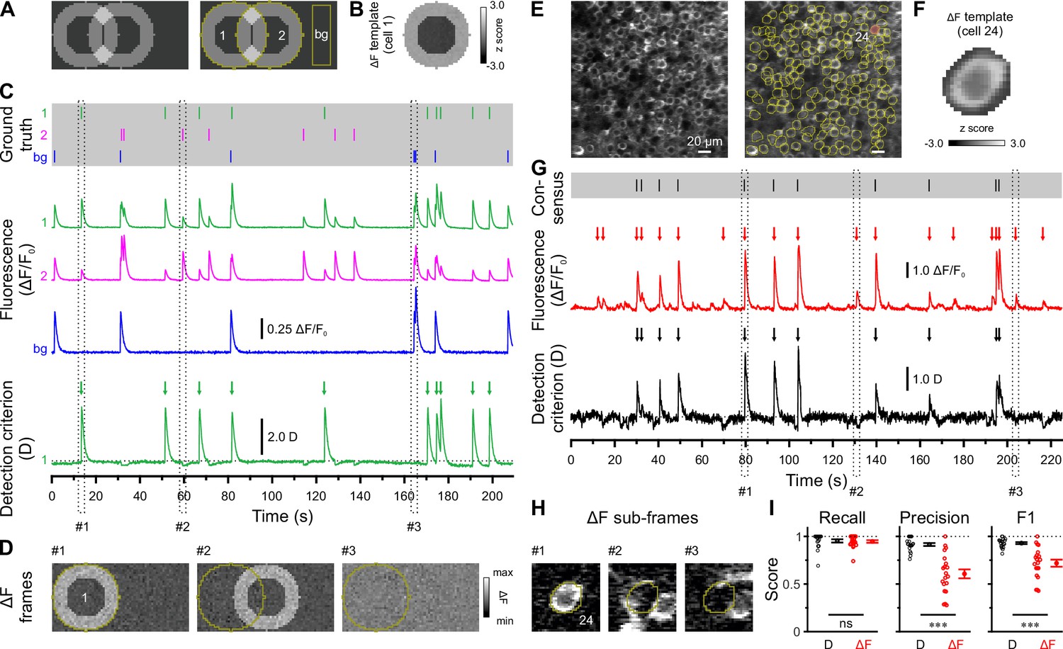
We used in vivo two-photon laser-scanning microscopy (2PLSM) in spontaneously breathing, head-fixed Emx1^IREScre:Rosa26^LSL-GCaMP6s mice to record somatic Ca²⁺ transients (CaTs) from CA1 PCs as a proxy of their firing activities. In this strain, Cre is expressed in virtually all CA1 PCs (Gorski et al., 2002; Kummer et al., 2012). Due to the finite point-spread function inherent to 2PLSM, dense cell labeling resulted in a non-negligible overlap of signals originating from neighboring somata and/or neurites. Our preliminary analysis revealed that standard CaT detection methods based on analyzing mean fluorescence intensities from regions of interests (ROIs) can lead to substantial false positive rates (Figure 1). Likewise, recent studies have demonstrated that popular CaT analysis algorithms can produce substantial misattribution errors under such conditions (Chen et al., 2020; Denis et al., 2020; Gauthier et al., 2022). We therefore devised a novel cell-specific spatial template-matching approach for the reliable detection of CaTs in densely labeled tissue, which we refer to as CATHARSiS (Calcium transient detection harnessing spatial similarity). CATHARSiS makes use of the fact that, for each cell, the spike-induced changes in GCaMP fluorescence intensity (ΔF) have a spatially inhomogeneous (ring-like) configuration (see Methods for details). In brief, a cell-specific spatial ΔF template representing the active cell is computed (Figure 1A and B) and optimally scaled to fit its ΔF in each recorded frame. Based on the optimum scaling factor and the quality of the fit, a detection criterion D(t) is computed for each time point (Clements and Bekkers, 1997). D(t) is then subjected to a general-purpose event detection routine for the extraction of CaT onsets (Rahmati et al., 2018). We first illustrate CATHARSiS by analyzing simulated spike-induced CaTs in ring-shaped cells (Figure 1A and B). Here, fluorescence signals of the cell of interest were contaminated by: (1) signals originating from a partially overlapping second cell, (2) spatially homogenous fluorescence changes mimicking axon-based neuropil activity (Kerr et al., 2005), and (3) a low level of Poissonian noise (Figure 1C). Figure 1C and D demonstrate that D(t) will increase only if ΔF has a spatial configuration similar to that of the template, i.e., if the simulated cell is active. Of note, D(t) is insensitive to a spatially uniform offset of ΔF and can decrease for mean ΔF increases having a dissimilar spatial configuration (#2 and #3 in Figure 1C and D). We applied CATHARSiS to two simulated sample cells of identical shape and varied their spatial overlap from 0 to 75% of the cell area, in accordance to the observed overlap in our empirical data. CATHARSiS correctly retrieved all ground-truth CaTs without false positive events (n=665 CaTs in total). We also found that the delay of the detected CaT onsets vs. simulated spikes was low (–0.3±0.0 frames), pointing to a high temporal accuracy of spike reconstruction, which is a prerequisite of a precise analysis of spatiotemporal activity patterns. We next evaluated CATHARSiS on data recorded from developing CA1 PCs in Emx1^IREScre:Rosa26^LSL-GCaMP6s mice in vivo (Figure 1E–I). For comparison, a consensus visual annotation by human experts was used (Figure 1G, top), as simultaneous electrophysiological data were not available (see Methods). We compared CATHARSiS to an event detection routine based on analyzing mean ΔF(t) and found that recall was ~95% for both approaches (Figure 1I; Supplementary file 1a). However, CATHARSiS yielded considerably fewer false positive events, thus resulting in a significantly higher precision and F1 score (Figure 1I). Importantly, the delay of detected CaT onsets relative to the consensus annotation was consistently low (0.9±0.1 frames at a frame rate of 11.6 Hz, n=20 cells), confirming that CATHARSiS achieved a high temporal accuracy.

Figure 1

Download asset Open asset

Calcium transient detection *har*nessing spatial similarity (CATHARSiS) enables reliable Ca²⁺ transient (CaT) detection in densely labeled tissue.

(A) Resting image of two partially overlapping simulated cells (*left*) and regions of interest (ROIs) used for analysis (*right*). bg – background. (B) ΔF template of cell 1. (C) Top, simulated trains of action potentials. Middle, relative changes from baseline fluorescence (ΔF/F₀) of ROIs shown in A. Bottom, detection criterion (D) for cell 1 and corresponding CaT onsets retrieved by CATHARSiS (arrows). (D) Sample ΔF images of three individual frames at time points indicated in C. Spikes in cells 1 or 2 translated into ring-shaped increases in ΔF, whereas those induced by bg spikes were applied to the entire field of view. (E) Resting GCaMP6s fluorescence image (*left*) and ROIs used for analysis (*right*). (F) ΔF template of the cell indicated in E. (G) Top, consensus visual annotation by two human experts for the same cell. Middle, ΔF/F₀ and detected event onsets (red arrows). Bottom, detection criterion (D) and corresponding CaT onsets retrieved by CATHARSiS (black arrows). (H) Sample ΔF images of three individual frames at time points indicated in G. Note that frames #2 and #3 led to false positive results if event detection was performed on mean ΔF, but not if performed on D. (I) Quantification of recall, precision, and F1 score for event detection based on D (i.e. CATHARSiS) and mean ΔF, respectively. Each open circle represents a single cell (n = 20 cells). Data are presented as mean ± SEM. ns – not significant. ^*** p<0.001. See also Supplementary file 1a and Figure 1—source data 1.

Figure 1—source data 1 Numerical data presented in Figure 1.: https://cdn.elifesciences.org/articles/82756/elife-82756-fig1-data1-v1.xlsx
Download elife-82756-fig1-data1-v1.xlsx

We conclude that CATHARSiS is suited for the reliable reconstruction of somatic CaTs in densely packed neuronal tissue with both high detection and temporal accuracies.

A transient period of firing equalization during CA1 development in vivo

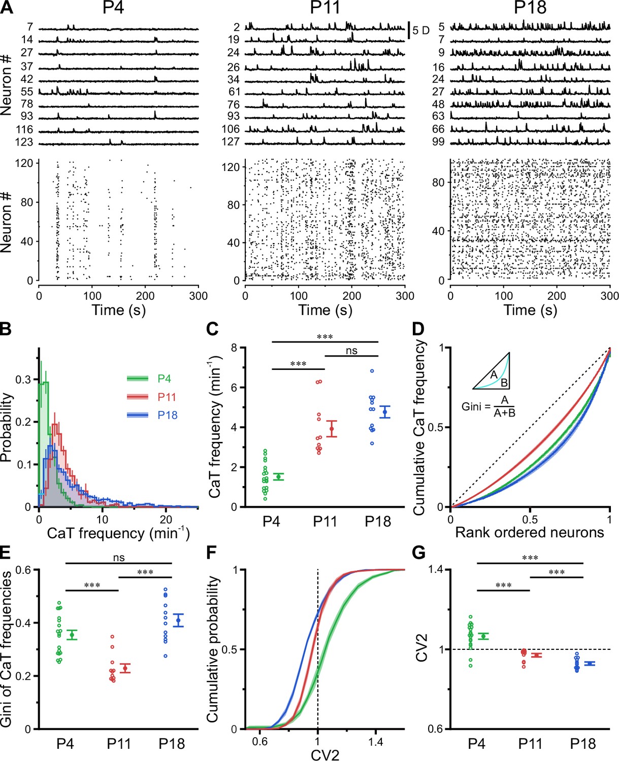
In the adult CA1, firing rate distributions are approximately log-normal, implying that a minority of neurons accounts for the majority of spikes. In addition, firing rates of individual cells are relatively stable across brain states and tasks, suggesting that skewed firing rate distributions reflect an inherent characteristic of mature hippocampal computations (Mizuseki and Buzsáki, 2013). To reveal developmental trajectories of single-cell activity, we applied CATHARSiS to extract spontaneous CaTs from Emx1+ PCs at P3–4 (n=19 fields of view [FOVs] from six mice), P10–12 (n=11 FOVs from six mice), and P17–19 (n=12 FOVs from six mice; Figure 2A). For the sake of brevity, these age groups are hereafter referred to as P4, P11, and P18, respectively. We found that mean CaT frequencies significantly increased ~2.5-fold from 1.5±0.2 min^–1 at P4 to 3.9±0.4 min^–1 at P11 and remained relatively stable afterward (P18: 4.8±0.3 min^–1, Figure 2B and C; see Supplementary file 1b). Additionally, we observed a striking change in the shape of CaT frequency distributions, which were broad and strongly right-tailed at P4 and P18, but much less so in the second postnatal week (Figure 2B; #6 in Supplementary file 1b). To quantify the dispersion of CaT frequencies among individual cells, we plotted the corresponding Lorenz curves (Figure 2D), in which the cumulative proportion of CaT frequencies is plotted against the cumulative proportion of cells rank-ordered by frequency (Mizuseki and Buzsáki, 2013). Here, the line of equality represents the case where all neurons have equal CaT frequencies. We computed the Gini coefficient as a measure of deviation from equality (for a graphical representation, see inset in Figure 2D). Gini coefficients underwent a transient minimum at P11, indicating that CaT frequencies among individual neurons were considerably more similar to each other as compared to P4 and P18 (Figure 2E). We next addressed whether developmental alterations in average CaT frequencies were accompanied by changes in their irregularity of occurrence. The local coefficient of variation (CV2), a robust measure of local spiking irregularity (Holt et al., 1996; Ponce-Alvarez et al., 2010), gradually declined from P4 to P18 (Figure 2G). At P11, CV2 was close to one, indicating that the irregularity of CaT occurrence is similar to that of a Poissonian point process, in which successive events occur independently of one another. As previously observed for CaT frequencies, CV2 distributions were also relatively broad at P4 and P18, but narrow at P11 (Figure 2F). Consistently, Gini coefficients of CV2 showed a distinct minimum at P11 (see #4 in Supplementary file 1b).

Figure 2

Download asset Open asset

A transient period of firing equalization during CA1 development in vivo.

(A) Sample *D(t*) traces (top) and raster plots showing reconstructed Ca²⁺ transient (CaT) onsets (bottom). Note the developmental transition from discontinuous to continuous network activity. (B) Empirical probability distribution of CaT frequencies. (C) Mean CaT frequencies per field of view (FOV). (D) Lorenz curves of CaT frequencies. Line of equality (dotted) represents the case that all neurons have equal CaT frequencies. Inset depicts Gini coefficient calculation. (E) Mean Gini coefficients per FOV. (F) Cumulative probability of mean coefficient of variation (CV2) of inter-CaT intervals. Note that, at P11, CV2 distribution is narrower and centered around 1. (G) Mean CV2 per FOV. For a Poisson process, CV2 = 1 (dotted line). Each open circle represents a single FOV. Data are presented as mean ± SEM. ns – not significant. P4: P3–4, n = 19 FOVs from six mice, P11: P10–12, n = 11 FOVs from six mice, P18: P17–19, n = 12 FOVs from six mice, and ^*** p<0.001. See also Supplementary file 1b and Figure 2—source data 1.

Figure 2—source data 1 Numerical data presented in Figure 2.: https://cdn.elifesciences.org/articles/82756/elife-82756-fig2-data1-v1.xlsx
Download elife-82756-fig2-data1-v1.xlsx

Collectively, our data reveal a transient equalization in CaT statistics of individual CA1 PCs during the second postnatal week, while highly skewed CaT frequency distributions eventually emerge only around/after eye opening.

CA1 undergoes a transient enhanced bursting period while progressively transitioning from discontinuous to continuous activity

Previous in vitro work has identified giant depolarizing potentials (GDPs) as the most prominent pattern of correlated network activity in the neonatal hippocampus (Ben-Ari et al., 1989; Garaschuk et al., 1998; Leinekugel et al., 1997). GDPs depend on a depolarizing action of GABA_A receptor-dependent transmission (Ben-Ari et al., 1989; Owens et al., 1996) and disappear at around the beginning of the second postnatal week, when GABA actions shift from mainly excitatory to mainly inhibitory (Tyzio et al., 2007; Yamada et al., 2004). To investigate whether a similar developmental profile of NB generation exists in the CA1 in vivo, we next determined the time-course of the fraction of active cells Φ(t) (Figure 3A). At P4, CA1 PCs spent relatively long time periods in a low-activity (silent) state, which was only interspersed by brief NBs (Figure 3A, left, and Figure 3B). During NBs, Φ(t) rarely exceeded 20% (Figure 3B), indicating that the degree of co-activation in vivo is considerably lower than that reported for GDPs in vitro (Flossmann et al., 2019; Garaschuk et al., 1998; Leinekugel et al., 1997). In contrast to GDPs, bursting activity in vivo was even more pronounced at P11, when the network tended to oscillate between a silent state and a bursting mode with an inter-burst period of ~2–10 s (Figure 3A, middle). We next asked if CA1 PCs could maintain non-zero activity for longer time periods. To this end, we partitioned recordings into non-overlapping 10-s-long windows, which we classified as either continuous or discontinuous based on a threshold criterion applied to Φ(t) (see Methods for details). Whereas network activity was found to be entirely discontinuous in the first postnatal week, CA1 started to dynamically transition between discontinuous and continuous activity at P11 (Figure 3A and C). At this age, the proportion of continuous activity was, on average, low but substantially increased toward P18 (Figure 3C and Supplementary file 1c).

Figure 3 with 1 supplement see all

Download asset Open asset

CA1 undergoes a transient enhanced bursting period while progressively transitioning from discontinuous to continuous activity.

(A) Sample traces of the fraction of active cells Φ(t). Gray and orange bars indicate discontinuous and continuous network activity, respectively. Bottom traces show time periods marked on top (dotted rectangle) at higher temporal resolution. Red dotted lines indicate the activity-dependent thresholds for network burst (NB) detection. (B) Empirical probability distribution of active cells per frame. (C) Continuous activity emerges at P11 and dominates over discontinuous activity at P18. (D) Power spectral density of Φ(t). (E) Bandpower of Φ(t) in the 0.1–0.5 Hz range. (F) The fraction of time that the network spends in NBs peaks at P11. (G) The average NB duration is lowest at P18. (H) Quantification of NB size as the mean fraction of active neurons (corrected for NB threshold as indicated in A). (I) Empirical probability distribution of the fraction of NBs that each cell is participating in. Each open circle represents a single field of view (FOV). Data are presented as mean ± SEM. ns – not significant. P4: P3–4, P11: P10–12, P18: P17–19, ^*** p<0.001, ^** p<0.01, and ^* p<0.05. See also Supplementary file 1c and Figure 3—source data 1.

Figure 3—source data 1 Numerical data presented in Figure 3.: https://cdn.elifesciences.org/articles/82756/elife-82756-fig3-data1-v1.xlsx
Download elife-82756-fig3-data1-v1.xlsx

To quantify developmental changes in the rhythmicity of network activity, we first computed the power spectrum of Φ(t). At P11, this revealed a distinct peak in the range of ~0.1–0.5 Hz (Figure 3D), pointing to the existence of a preferred oscillation frequency of CA1 PCs. Such a power peak was absent at P4 and reduced at P18. Accordingly, band power in the 0.1–0.5 Hz frequency range was significantly higher in the second postnatal week than at earlier or later stages (Figure 3E).

To characterize periods of neuronal co-activation in more detail, we next extracted NBs by thresholding Φ(t). NB thresholds were determined separately for each FOV using surrogate data, accounting for differences in CaT frequencies (Figure 3A, bottom, and Methods). The fraction of time that the network spent in NBs was lowest at P4 and peaked at P11 (Figure 3F). Moreover, NBs at P18 were significantly shorter in duration than during the first and second postnatal weeks (Figure 3G). We quantified NB size as the fraction of active cells (corrected for the threshold applied to Φ[t]) and found that it only declined after P11 (Figure 3H). At P11, each neuron participated in 14.4 ± 1.2% of all NBs, which significantly exceeded participation rates at P4 (10.3 ± 0.8%) and P18 (11.2 ± 0.4%; see #6 in Supplementary file 1c). Importantly, these developmental changes in NB characteristics were robust to a wide range of NB definitions (Figure 3—figure supplement 1 and Methods). Additionally, distributions of participation rates were relatively narrow at P11 (Figure 3I), pointing to a greater similarity of cells with respect to their contribution to NB generation as compared to earlier or later developmental stages (#7 in Supplementary file 1c).

Taken together, our data reveal that CA1 undergoes a transient period of enhanced bursting activity that coincides with the developmental appearance of continuous activity states during the second postnatal week. At this age, network activity displays rhythmicity in the sub-Hz range – in spite of the close-to-random activation of individual PCs.

Enhanced population coupling underlies network burstiness in the second postnatal week in vivo

The transient developmental increase in bursting propensity was unexpected, as (1) GDPs in vitro disappear soon after the first postnatal week (Ben-Ari et al., 1989; Garaschuk et al., 1998; Khazipov et al., 2004) and (2) previous in vivo data from neocortex revealed a reduction in correlated network activity during the same time period (Colonnese et al., 2010; Golshani et al., 2009; Rochefort et al., 2009; van der Bourg et al., 2017). We therefore assessed whether the enhanced burstiness at P11 reflects an increase in functional neuronal coupling. We first investigated the coupling of single-cell activity to that of the overall population. For each cell, we computed its population coupling (PopC) index (Okun et al., 2015; Sweeney and Clopath, 2020) and tested for its significance using surrogate data (see Methods). The PopC index significantly peaked at P11 (Figure 4A, Supplementary file 1d), while there was no difference between P4 and P18. The higher PopC index at P11 arose from a significantly higher fraction of coupled cells (Figure 4B), whereas the indices of significantly coupled cells were similar (Figure 4C). We next addressed whether the increased PopC index at P11 results from an increase in pairwise temporal correlation of CaTs. To this end, we computed the spike-time tiling coefficient (STTC) as a frequency-independent affinity metric of two event time series (Cutts and Eglen, 2014; Figure 4D). The fraction of significantly correlated cell pairs did not significantly differ between P4 and P11 (P4: 13 ± 2% and P11: 23 ± 5%), but strongly decreased to 5 ± 1% at P18 (Figure 4E). STTCs of significantly correlated pairs profoundly declined from 0.18±0.01 at P4 to 0.09±0.01 already at P11, but did not significantly change afterward (P18: 0.10±0.00; Figure 4F and G). These data suggest that developmental changes in pairwise neuronal correlations do not account for the increased PopC or the increased burstiness of CA1 PCs during the second postnatal week. We further analyzed the spatial structure of CA1 ensemble dynamics. We found that the dependence of STTCs on the Euclidean somatic distance was weak already during the first two postnatal weeks and non-significant at P18 (Figure 4H), indicating that the horizontal confinement of patterned network activity is weak or absent throughout the developmental period studied here.

Figure 4

Download asset Open asset

Enhanced population coupling (PopC) underlies network burstiness in the second postnatal week in vivo.

(A) The mean PopC index peaked at P11. (B) Mean fraction of cells with significant PopC. (C) Mean PopC index of significantly coupled cells only. (D) Sample spike-time tiling coefficient (STTC) matrices (re-ordered) from three individual fields of view (FOVs) at P4, P11, and P18. (E) Mean fraction of cell pairs having a significant STTC. (F) Cumulative probability of STTCs of significantly correlated cell pairs only. (G) Mean STTCs of significantly correlated cell pairs. (H) Relationship between STTC and Euclidean somatic distance for significantly correlated cell pairs. ρ denotes the Spearman’s rank correlation coefficient for all cell pairs analyzed (n) at a given age. (**A–C** and **E–G**) Each open circle represents a single FOV. Data are presented as mean ± SEM. ns – not significant. P4: P3–4, P11: P10–12, P18: P17–19, ^*** p<0.001, and ^** p<0.01. See also Supplementary file 1d and Figure 4—source data 1.

Figure 4—source data 1 Numerical data presented in Figure 4.: https://cdn.elifesciences.org/articles/82756/elife-82756-fig4-data1-v1.xlsx
Download elife-82756-fig4-data1-v1.xlsx

Collectively, our data reveal that enhanced network burstiness during the second postnatal week is associated with a higher fraction of cells significantly locked to the activity of the local network, while pairwise neuronal correlations are low.

Motifs of CA1 network activity undergo distinct developmental alterations

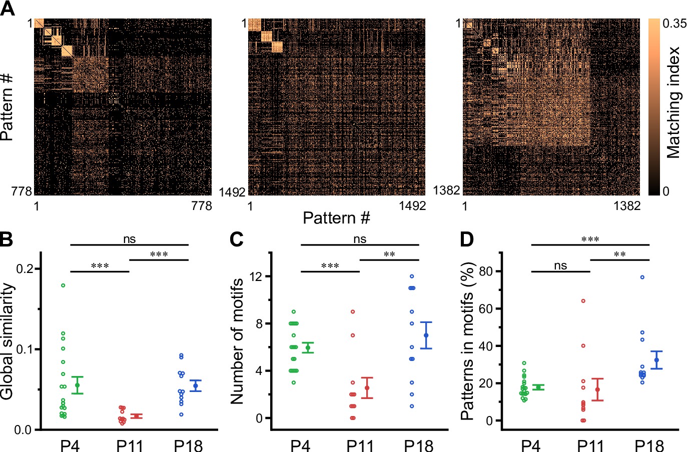
Recurring spatiotemporal cellular activation patterns are a hallmark of network activity in the adult hippocampus in vivo (Villette et al., 2015). Whether such repeating patterns (hereafter referred to as ‘motifs’) are already present at early developmental stages is unknown. To detect motifs, we divided the recording time into non-overlapping bins, each represented by a binary spatial pattern (vector) of active and inactive cells, followed by computing the matching index matrix of all possible pattern pairs (Figure 5A). We then applied an eigendecomposition-based clustering method to each similarity matrix in order to detect potential motifs, while testing for their significance using surrogate data (see Methods). First, this analysis revealed that the global similarity of the activation patterns was lowest at P11 (Figure 5B, Supplementary file 1e), whereas it was similar between P4 and P18. This finding implies that there is less commonality between the sets of active cells present in different patterns at P11 and, thus, more random recruitment of cells. Furthermore, the number of motifs was significantly lower at P11 (2.5±0.9) as compared to P4 (5.9±0.4) and P18 (7.0±1.1; Figure 5C). When computing the fraction of patterns belonging to each motif, we found that the motifs had the highest repetition rate at P18 (32.0 ± 4.7%), while there was no significant difference between P4 (17.8 ± 1.2%) and P11 (16.6 ± 5.9%; Figure 5D). The increase in motif repetition rate toward P18 suggests that recurring cellular activation patterns become more stable only after the onset of environmental exploration.

Figure 5

Download asset Open asset

Motifs of CA1 network activity undergo distinct developmental alterations.

(A) Similarity matrices (matching index) of binary activity patterns (re-ordered for illustration of motif detection) from three individual fields of view (FOVs) at P4, P11, and P18. (B) Global similarity of activity patterns is lowest at P11. (C) The absolute number of detected motifs per FOV is lowest at P11. (D) Motif repetition quantified as the fraction of activity patterns belonging to each motif. Each open circle represents a single FOV. Data are presented as mean ± SEM. ns – not significant. P4: P3–4, P11: P10–12, P18: P17–19, ^*** p<0.001, and ^** p<0.01. See also Supplementary file 1e and Figure 5—source data 1.

Figure 5—source data 1 Numerical data presented in Figure 5.: https://cdn.elifesciences.org/articles/82756/elife-82756-fig5-data1-v1.xlsx
Download elife-82756-fig5-data1-v1.xlsx

Effects of nitrous oxide on body movements, vital parameters, and network dynamics

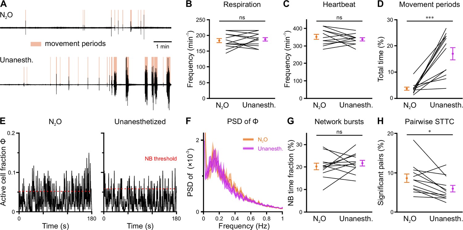
In an attempt to reduce spontaneous movements and thus increase mechanical stability during two-photon imaging, all measurements discussed so far were performed in the presence of the analgesic-sedative nitrous oxide, following our established procedures in neonatal mice (Kirmse et al., 2015). However, general anesthetics can have a profound impact on brain activity in an age- and dose-dependent manner (Ackman and Crair, 2014; Chini et al., 2019; Cirelli and Tononi, 2015; Yang et al., 2021). As the effects of nitrous oxide on neuronal dynamics in the developing CA1 had been unknown, we performed a separate set of experiments (n=12 FOVs from six mice) in which we compared nitrous oxide to unanesthetized conditions using a paired design at P11 (Figure 6—figure supplement 1). Nitrous oxide reduced the time that mice spent in locomotion periods by several-fold (Figure 6A and D and Figure 6—figure supplement 1, Supplementary file 1f) and, hence, minimized periods of z-drift that needed to be discarded from analysis in two-photon Ca²⁺ imaging. Unlike most conventional anesthetics, however, nitrous oxide did not affect respiration or heart rate (Figure 6B and C and Figure 6—figure supplement 1). To prevent photo-bleaching in these longer-lasting experiments, we minimized the laser power and increased the detector gain, which effectively reduced the signal-to-noise ratio in CaT detection. We observed slightly higher mean CaT frequencies in unanesthetized mice (Figure 6E, Figure 6—figure supplement 2B and C), while the Gini coefficient of CaT frequencies was unaffected (Figure 6—figure supplement 2D). The time the network spent in continuous activity was similarly low (Figure 6—figure supplement 2E), and the oscillatory dynamics of CaTs (Figure 6F and Figure 6—figure supplement 2F) and NB properties (Figure 6G and Figure 6—figure supplement 2G) were unaltered. The most consistent effect of nitrous oxide was an increase in the percentage of correlated neuron pairs (Figure 6H), whereas their STTC values were unaffected (Figure 6—figure supplement 2H). This further translated into a higher fraction of cells that are significantly locked to local CA1 activity under nitrous oxide as compared to unanesthetized conditions (Figure 6—figure supplement 2I).

Figure 6 with 2 supplements see all

Download asset Open asset

Effects of nitrous oxide (N₂O) on body movements, vital parameters, and network activity at P11.

(A) Sample respiration/movement signal from an individual mouse receiving either 75% N₂O/25% O₂ (top) or pure O₂ (Unanesth., bottom). Detected movement periods are highlighted. (B) Respiration rate is unaffected by N₂O (n = 12 fields of view [FOVs] from six mice). (C) Heart rate is unaffected by N₂O (n = 11 FOVs; in the recording from one FOV, heart rate could not be reliably determined). (D) N₂O significantly reduces movement periods. (E) Sample traces of the fraction of active cells Φ(t) (Δt = 3 frames). Red dotted lines indicate the activity-dependent thresholds for network burst (NB) detection. (F) Power spectral density of Φ(t) is similar in the presence or absence of N₂O. (G) The fraction of time that the network spends in NBs. (H) Fraction of neuron pairs having a significant spike-time tiling coefficient (STTC). Data are presented as mean ± SEM. ns – not significant. ^*** p<0.001 and ^* p<0.05. See also Supplementary file 1f and Figure 6—source data 1.

Figure 6—source data 1 Numerical data presented in Figure 6 and Figure 6—figure supplement 2.: https://cdn.elifesciences.org/articles/82756/elife-82756-fig6-data1-v1.xlsx
Download elife-82756-fig6-data1-v1.xlsx

In sum, nitrous oxide moderately reduces pairwise and population coupling of CA1 PCs, whereas network burstiness and continuity resemble those observed in unanesthetized mice. A major advantage of nitrous oxide lies in the reduction of extended movement periods, which significantly increases mechanical stability during two-photon imaging.

A neural network model with inhibitory GABA identifies intrinsic instability dynamics as a key to the emergence of NBs

Hitherto our analyses of experimental data revealed an unexpected bursting behavior of CA1 PCs at P11, despite the developmental emergence of synaptic inhibition (Murata and Colonnese, 2020; Spoljaric et al., 2017; Tyzio et al., 2007), which we related to their higher coupling to local network activity. However, the mechanisms governing in vivo network burstiness as well as its functional implications remain to be understood. Here, we provide mechanistic insights into these open questions by using computational network modeling and stability analysis techniques.

We employed a recurrent neural network (RNN) model of mean firing-activity rates of excitatory glutamatergic (PC) and inhibitory GABAergic (IN) cell populations ( $A_{PC}$ and $A_{IN}$ ) with dynamic synaptic weights (Flossmann et al., 2019; Rahmati et al., 2017; Figure 7A). Here, we constrain the model with previously reported and our present experimental data obtained for P11: (1) GABAergic synapses are considered to be inhibitory (Kirmse et al., 2015; Murata and Colonnese, 2020; Valeeva et al., 2016) and (2) the spontaneous time-averaged $A_{PC}$ is effectively non-zero (Figure 2C). We found that such a network operates under a bi-stable regime, where two stable spontaneous fixed points (FPs) exist: one at a silent state ( $A_{PC} = A_{IN} = 0$ Hz) and the other at an active state ( $A_{PC} \neq 0$ Hz and $A_{IN} \neq 0$ Hz; green dots in Figure 7B). This is reminiscent of our experimental observations demonstrating that CA1 dynamically transitions between discontinuous and continuous activity states at this stage (see Figure 3A–C). The ability of the network model to embed the FP at an active state is mainly due to the stabilization function of inhibitory GABA (Latham and Nirenberg, 2004; Rahmati et al., 2017). Strikingly, our simulations showed that the network can process a given input quite differently at the silent and active states, respectively (time points a and c in Figure 7C). To this end, we applied a set of two excitatory inputs to the network’s PC and IN populations ( $e_{PC}$ and $e_{IN}$ ), resembling, e.g., SPW-driven inputs to CA1 (Figure 7C). We set the input strengths and duration to be identical across the two states. We found that, when operating at the active state, the network activity monotonically decays back to this state, once the input ceases (a in Figure 7C). However, at the silent state, input removal is followed by a transient profound surge in network activity (c in Figure 7C). Hereafter, we refer to this supra-amplification activity as simulated NB (simNB), emulating experimentally observed NBs (Figure 3).

Figure 7

Download asset Open asset

A neural network model with inhibitory GABA identifies intrinsic instability dynamics as key to the emergence of network bursts.

(A) Schematic diagram of the short-term synaptic plasticity (STP)-recurrent neural network (RNN) model. (B) The $A_{IN} - A_{PC} -plane$ of the full STP-RNN’s stationary dynamics. Note the presence of two stable fixed points (FPs; green dots) at silent and active states as well as the unstable FP (black dot). (C) Simulated network burst (simNB) generation requires network silencing. The model was stimulated by pulse-like input to both pyramidal cell (PC) and interneuron (IN) populations for a duration of 0.020 s (at t = 3 and 9.2 s: $e_{PC} = e_{IN} = 0.25$ ; at t = 8 s:, $e_{PC} = 0.25$ $e_{IN} = 0.75$ ). Zoom-in of the activity around the stimulation times at active (a and b) and silent (c) states is shown in right panels. Input time series are shown on top of the plots. (D) The presence of an amplification domain in the initial phase of network firing dynamics enables the emergence of simNBs. The $A_{IN} - A_{PC} -plane$ of the STP-RNN with synaptic efficacies frozen at active (a, top) and silent (b, bottom) states, right before input arrival. (**E–G**) Transition from active to silent state requires specific input ratios. Input delivered at t = 8 s. (E) A failed transition: $e_{PC} = 0.25$ , $e_{IN} = 0.5$ (F) A successful transition: $e_{PC} = 0.25$ , $e_{IN} = 1$ . (G) A color-coded matrix of successful (dark green) and failed (light green) transitions to the silent state in response to different combinations of $e_{PC}$ and $e_{IN}$ amplitudes. (**H–J**) Both the transition from the silent to the active state and the simNB generation require specific input ratios. Input delivered at t = 9.2 s. Same as **E–G**, but for the backward transition to the active state. +simNB and –simNB indicate the emergence and absence of bursts.

Network state-dependency of simNB generation

To disclose the mechanisms underlying this distinct behavior of the network at the silent and active state (Figure 7C), we computed the corresponding steady-state $A_{IN} - A_{PC} -plane$ of the network, after freezing the slow short-term synaptic plasticity (STP) dynamics and, thus, synaptic weights (frozen STP-RNNs), at either of these states separately (Figure 7D). This analysis enables assessing the initial phase of network activity following an input perturbation. We found that, while operating at the silent state, the active state is not initially accessible to the network (lower panel in Figure 7D). Instead, an unstable FP is present in the network’s fast (i.e. firing activity) dynamics, which builds an amplification threshold around the attraction domain of the FP located at the silent state. This in turn allows for the emergence of simNBs. A sufficiently strong perturbation, amenable to initially push the network activity beyond this threshold (i.e. to the amplification domain), will transiently expose the network to its intrinsic instability-driven dynamics, thereby effectively triggering a simNB (c in Figure 7C). Note that this unstable FP is different from its counterpart in the full system (Figure 7B) and is only visible in the network’s fast dynamics. In particular, this FP is transient and disappears around the peak of the elicited simNB, mainly due to short-term synaptic depression (Rahmati et al., 2017). Unlike the silent state, the network frozen at the active state has no amplification domain, but instead two attraction domains related to its FPs at silent and active states (upper panel in Figure 7D). This explains the network’s incapability of eliciting simNBs when operating at the active state. Collectively, these results suggest that simNBs, initiated by the input, are mainly an expression of the network’s intrinsic instability dynamics, where the silent periods of the network are a prerequisite for its emergence. The model behavior agrees with our experimental data revealing both prominent burstiness and a dominance of discontinuous activity at P11 (see Figure 3A–C).

Input-strength dependency and internal deadline of state transitions

What are the input requirements that allow the network to transition between the active and the silent states? First, we found that silencing the network from an active state requires specific ratios of excitatory input strengths to be delivered to its PC and IN populations (Figure 7E–G). In particular, the presence of GABAergic inhibition can effectively promote this transition, where otherwise a relatively much stronger $e_{PC}$ is required to silence the network solely (Figure 7G). Furthermore, once silenced, pushing the network back to its active state is also dependent on input ratio (Figure 7H–J). However, to make such a transition, the network becomes noticeably more selective about the input ratio (compare Figure 7G and J). For both transitions, the proper ratios of the inputs are effectively determined by the approximated initial phase of the network response (Figure 7D), and thus mainly dependent on the synaptic weights right before the input arrival. In sum, these results suggest that proper input strengths onto the PC and IN populations, along with the inhibitory action of GABA, play key roles in the dynamic state transitioning of the network, thereby allowing for its burstiness.

Considering the dynamics of synaptic weights in our model along with their significance for state transitions, we next investigated the impact of input timing (Figure 8). We found that, once silenced by the first input, a deadline is formed for the network’s transitioning back to the active state (dotted line in Figure 8A, D, G and H). If the second input misses the deadline, the network will elicit a large-amplitude simNB but is not able to converge to the active state any longer (Figure 8D). Prior to this deadline and depending on the input ratio (Figure 7J), the network will either transition to the active state (Figures 8A and 7H) or return to the silent state (Figure 7I). Importantly, our analysis showed that this deadline is an internal property of the network and cannot be overruled by any input level (see below). Therefore, specific combinations of input ratio (Figure 7J) and input timing (Figure 8G) are required for transitioning to the active state. In addition, once the simNB failed to converge to the active state, the network will encounter a new deadline (Appendix 1 and Figure 8—figure supplement 1). In sum, these results imply that the silent state of the network can have per se different hidden sub-states, each with a specific input-encoding operating scheme.

Figure 8 with 1 supplement see all

Download asset Open asset

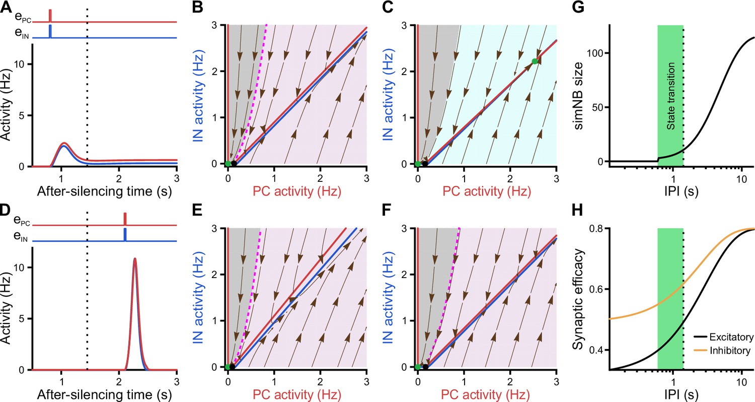
Internal deadline of state transitions.

(**A–C**) Input delivered to the network before the deadline can move it to active state. (A) A successful transition. The input delivered at t = 0.8 s; $e_{PC} = 0.25$ , $e_{IN} = 0.25$ . (B) The $A_{IN} - A_{PC} -plane$ of the short-term synaptic plasticity (STP)-recurrent neural network (RNN) with synaptic efficacies frozen at the silent state right before the input arrival. (C) Same as B, but frozen at the peak of the network burst (i.e. simulated network burst [simNB]) shown in A. Note the presence of the transient stable fixed point (FP; non-origin green dot), which triggers the transitioning to the active state. (**D–F**) Once the deadline is missed, the network cannot be moved to the active state by the subsequent input. Same as A–C, but the input delivered at t = 2.1 s. Note the absence of a non-origin transient stable FP in F, in contrast to C. (G) The simNB size and network transition to the active state depend on the inter-pulse intervals (IPIs: the arrival time of the next input relative to the silencing time of the network). simNB size is computed as the maximum of $A_{IN} + A_{PC}$ after the secondary input. Note the presence of a short window for transitioning to the active state. $e_{PC} = 0.25$ , $e_{IN} = 0.25$ . (H) Same as G, but for the non-scaled efficacies of GABAergic ( $u_{I} x_{I}$ ; orange; see Methods) and glutamatergic ( $u_{p} x_{P}$ ; black) synapses, right before the arrival of the secondary input. (**A, D, G, and H**) The dotted line at t = 1.45 s depicts the internal deadline.

Having found the intrinsic deadline as a main determinant for the type of NB, we next investigated the origin of these different activity patterns. How does the network decide between transitioning to the active state and returning to the silent state? Remarkably, we found that the deadline for network transitioning to the active state is mechanistically dependent on the presence of a transient stable FP in its fast dynamics around the peak of the simNB. This can be seen in the two examples where the network receives the same input but at different inter-pulse intervals (IPIs), one preceding (Figure 8A–C) and the other exceeding the deadline (Figure 8D–F). For both IPIs, at the time right before the second input (Figure 8B and E), the frozen RNNs only provide evidence for the emergence of simNB, but not for the state transition (note the presence of an amplification domain; pink area). Importantly, we found, however, that in the case of the shorter IPI, the network is able to form a transient, stable non-zero FP in its frozen RNN, at the peak of the simNB (compare Figure 8C and F). This FP can transiently attract the network’s activity toward itself, and as the activity evolves accordingly, it also changes its position in the corresponding updated frozen STP-RNN, until eventually converging to its counterpart in the full system. Intuitively, this transient, stable FP can guide the network’s activity toward that of the full system (see the non-origin green dot in Figure 7B). The temporal repositioning of this stable FP is due to the activity-dependency of the synaptic weights in our model. Besides, our findings show that the existence of this FP around the simNB peak is effectively determined by simNB size (Figure 8G). If simNB size exceeds an internally determined threshold, the network cannot build such a transient stable FP due to a reduction of synaptic weights (Rahmati et al., 2017); consequently, the simNB will be attracted toward the silent state. In this line, Figure 8G shows that simNB size is effectively determined by the IPI. The longer the IPI (thus, the silent period) is, the larger the simNB will be. Here, the IPI-dependency of the simNB size mainly reflects the slow recovery from short-term depression of excitatory synapses at the silent state (Figure 8H).

In conclusion, our modeling results indicate that developing CA1 possesses multiple input-encoding schemes, which are effectively determined by three factors: (1) the input ratio, (2) the input timing, and (3) the non-linearity and dynamics of synaptic weights.

A bi-stable STP-RNN model with inhibitory GABA robustly explains our experimental observations

We next investigated whether alternative network models (or mechanisms) are better suited to explain the observed CA1 dynamics in the second postnatal week. By decreasing the population-activity thresholds (θ) and/or changing the polarity of GABAergic synapses from inhibitory to excitatory, we created two operationally distinct models called Mono-RNNi (θ_PC↓, ‘i’ for inhibitory GABA) and Mono-RNNe ( $J_{IN} \to - 0.5 \times J_{IN}$ , θ_PC↓, θ_IN↓; ‘e’ for excitatory GABA; Figure 9—figure supplement 1A). Of note, lower θ reflects a higher background input to, or a lower spike threshold of, the neuronal population (see Methods). Each of the models is mono-stable with one spontaneous FP in an active state (non-origin green dots in Figure 9—figure supplement 1A).

As a prerequisite for comparison, both Mono-RNNi and Mono-RNNe can generate silent periods, simNBs, and an active state with $A_{PC} > 0$ (Figure 9—figure supplement 1B–F), as observed in our data. As compared to the bi-stable STP-RNN model (Figure 7 and Figure 9—figure supplement 1A), however, both mono-stable networks are less plausible in explaining our experimental observations for several reasons. First, due to the lack of a silent FP, Mono-RNNi and Mono-RNNe can transition to and remain in a silent state only in the (continuous) presence of synaptic input (Figure 9—figure supplement 1C and D). Second, for silencing ( $A_{PC} = A_{IN} = 0$ ), the external input to at least one of the populations needs to be inhibitory (Figure 9—figure supplement 1E, green areas). However, input to CA1 at this age is mainly mediated by glutamatergic projections from entorhinal cortex and CA3. In addition, considering inhibitory input violates the assumption of excitatory GABAergic synapses in the Mono-RNNe. Third, both Mono-RNNi and Mono-RNNe require a relatively long silencing (of at least the PC population) to effectively generate simNBs (Figure 9—figure supplement 1F), which is difficult to reconcile with the time-course of SPWs (tens of milliseconds).

The intrinsic bi-stability of the STP-RNN renders it computationally different from the mono-stable alternatives: (1) In the STP-RNN, simNBs are triggered by suitable inputs (Figures 7 and 8), whereas in Mono-RNNi and Mono-RNNe, simNBs are elicited in the form of rebound bursts only after the cessation of the non-specific silencing inputs (Figure 9—figure supplement 1C, D and F). This feature renders the STP-RNN potentially more suitable for input discrimination prior to the onset of environmental exploration. (2) Regardless of their size, rebound simNBs will always return to the active state in Mono-RNNi and Mono-RNNe (Figure 9—figure supplement 1C and D), in contrast to the STP-RNN, which may also return to its rest state (Figures 7 and 8). (3) Mono-RNNe lacks an inhibition-stabilized network (ISN) regime (Figure 9—figure supplement 1A), which is thought to provide a general strategy for supporting more complex computations (Latham and Nirenberg, 2004; Tsodyks et al., 1997).

In sum, these results indicate that the proposed STP-RNN, operating under bi-stability, is not only computationally more flexible but also more plausible in explaining our experimental observations.

Inhibitory stabilization of a persistent active state in the bi-stable STP-RNN model

Using our STP-RNN model, we further investigated the functional significance of the network behavior during the second postnatal week. Our analyses show that an ISN regime is effectively accessible at this age due to the developmental increase of synaptic inhibition (Figure 9A and B). This presumably enables CA1 to process more complex computations (while avoiding instabilities) in parallel to the developmental strengthening of sensory inputs. Importantly, the active state in our model is also located in the ISN FP-domain (Figure 9—figure supplement 1A, left). Such an ISN regime is absent if GABAergic transmission is excitatory (Figure 9A [right] and Figure 9B). Moreover, the developmental increase in the strength of synaptic inhibition ( $J_{IN}$ ) enables the network to operate as an ISN at a wider range of PC activity levels (Figure 9C). This is because the unstable FP-domain, confined to low levels of PC activity, is progressively replaced by the ISN FP-domain as inhibitory synapses become stronger (Figure 9A and B). In the model, simNB size is reduced by a strengthening of inhibition (akin to our experimental observations at P11 vs. P18), but increased if GABA is considered excitatory (unlike our data at P11 vs. P4; Figure 9D). This implies that the changes in inhibitory strength alone are unsuited to explain the enhanced burstiness in the second postnatal week. We found, however, that the experimentally reported, concurrent developmental strengthening of glutamatergic synapses ( $J_{PC}$ ; for review see Kirmse and Zhang, 2022) exerts an opposite effect by profoundly amplifying simNBs (Figure 9E). Collectively, our analyses portend that the emergence of a persistent active state in CA1 reflects the developmental strengthening of both GABAergic inhibition ( $J_{IN}$ ) and glutamatergic excitation ( $J_{PC}$ ) as well as changes in background input and/or intrinsic excitability (θ). In line with this, the enhanced burstiness at P11 is an expression of the complex neural dynamics in a bi-stable STP-RNN that identify the second postnatal week as a key transitional period in CA1 network maturation.

Figure 9 with 1 supplement see all

Download asset Open asset

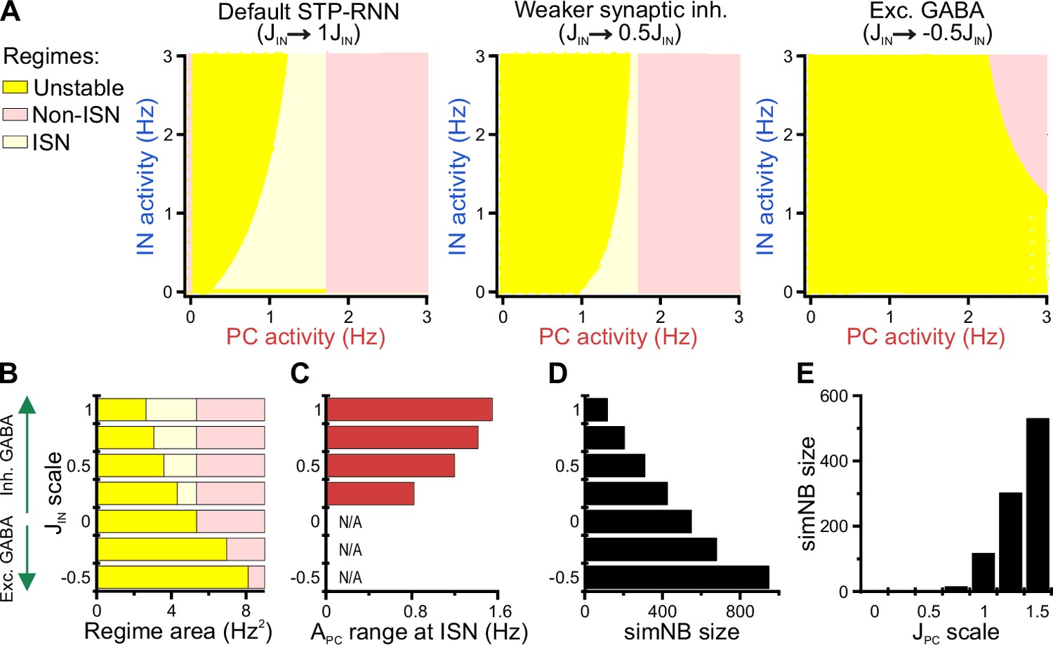
Inhibitory stabilization of a persistent active state in the bi-stable short-term synaptic plasticity (STP)-recurrent neural network (RNN) model.

(A) The inhibition-stabilized network (ISN) regime becomes accessible to the network upon the developmental emergence of synaptic inhibition. The colored regions in each $A_{IN} - A_{PC} -plane$ of the network model depict the fixed point (FP)-domains of three possible operating regimes: unstable dynamics, ISN, and Non-ISN. Synaptic inhibition strength $J_{IN}$ was set to 3 (inhibitory; left), 1.5 (inhibitory, middle), and –1.5 (excitatory, right). (**B–D**) Effect of strength and polarity of GABAergic synapses ( $J_{IN}$ ) on the availability of the ISN regime (B), the maximum range of pyramidal cell (PC) activity in the ISN regime (C), and size of simulated network bursts (simNBs) when triggered at the rest state (D). Results were obtained by scaling $J_{IN}$ in the STP-RNN model with values indicated on the y-axis. The area of each operating regime was computed based on the area of its FP-domain in the $A_{IN} - A_{PC} -plane$ (with limits as in A). (E) Dependency of simNB size on the strength of glutamatergic synapses ( $J_{PC}$ ). Default value of $J_{PC}$ in STP-RNN was 6.5 (corresponding to a scale of 1).

Discussion

Developmental trajectories of network dynamics in CA1 in vivo

Our data demonstrate that the activity of CA1 PCs in the first postnatal week is generally low and exclusively discontinuous in nature, as they spend most of the time in a silent rest state that is only interrupted by relatively brief NBs (Figures 2A–C ,–3A–C). In other words, CA1 PCs are incapable of sustaining persistent activity at this age, similar to findings in visual cortex (Ackman et al., 2012; Hanganu et al., 2006; Kirmse et al., 2015; Kummer et al., 2016). Previous data-driven computational modeling further showed that such dynamics can be emulated by mono-stable network models, in which excitatory GABA effectively promotes network burstiness (Flossmann et al., 2019). CA1 NBs differ from their neocortical counterparts in that the latter exhibit a distinct horizontal confinement that appears to be largely absent in CA1. This is evident in the weak distance-dependency of pairwise correlations of CA1 PCs (Figure 4H), extending previous results from large-scale imaging (Graf et al., 2021) and electrophysiological (Valeeva et al., 2019; Valeeva et al., 2020) studies. Whether differences in spatial properties of NBs in neocortex vs. hippocampus reflect their specific input characteristics and/or connectivity patterns is an open question. Likewise, the developmental relevance of such differences is unknown. However, wavefront-containing activity patterns have been causally linked to the developmental refinement of topographic maps (Cang et al., 2005; Li et al., 2013) and receptive field characteristics (Albert et al., 2008; Wosniack et al., 2021) in the visual cortex, suggesting that their absence in CA1 might reflect the lack of a clear topical macro-organization of the hippocampus (Bellistri et al., 2013).

We here identify the second postnatal week as a key transitional period in CA1 network maturation. For the first time in development, CA1 PCs are able to maintain spontaneous persistent activity, while this transition toward embedding continuous activity is largely completed by P18 (Figure 3A–C). In the second postnatal week, when discontinuous activity still dominates (Figure 3C), CA1 PCs undergo a transient period of enhanced network burstiness (Figure 3A). This trajectory markedly differs from what has been previously reported for the hippocampus in vitro, where GDPs disappear shortly after the first postnatal week. At this time, GABA-releasing INs already inhibit CA1 PCs (Murata and Colonnese, 2020; Spoljaric et al., 2017; Tyzio et al., 2008), implying that NBs in vivo do not depend on GABAergic excitation (in contrast to GDPs). NBs are also observed at P18, but these are short in duration (Figure 3G) and recruit fewer neurons (Figure 3H) than at earlier stages. Strikingly, whereas NBs at P11 are large and frequent, repetition rates of recurring cellular activation patterns (a prime characteristic of adult hippocampal activity) significantly increased only after the onset of environmental exploration (Figure 5D). This was accompanied by highly skewed firing rate distributions at P18 (quantified as CaT frequencies; Figure 2B–E). The latter are thought to underlie sparse coding (Ikegaya et al., 2013; Narayanan and Johnston, 2012; Roxin et al., 2011; Trojanowski et al., 2020; Yassin et al., 2010), an energy-efficient regime of input processing and information storage (Mizuseki and Buzsáki, 2013). Collectively, our data indicate that CA1 network activity acquires a number of ‘adult-like’ characteristics by P18, i.e., shortly after the onsets of pattern vision, active whisking, and environmental exploration. At P11, prominent network burstiness and emergent continuity were also observed in unanesthetized mice (Figure 6), confirming that they did not result from the use of nitrous oxide. However, further investigations are warranted, as potential age- and state-dependent effects of nitrous oxide on neuronal dynamics are currently unknown. This might be particularly relevant in the context of the emergence of an active sleep-wake cycle around eye opening (see also Chini et al., 2019; Shen and Colonnese, 2016).

A role for intrinsic network instability and synaptic inhibition in NB generation in CA1

During the transition period (i.e. P11), bursting activity exhibited a preferred frequency of ~0.1–0.5 Hz, indicating that NBs occur in a temporally non-random manner (Figure 3). However, individual neurons were recruited more randomly at this age, as the number of significant motifs of network activity as well as their average repetition probability were lowest (Figure 5). At P11, the occurrence of CaTs in individual cells resembled a Poissonian process (Figure 2), and pairwise neuronal correlations were lower than at P4 (Figure 4G). We here set out to explain these seemingly discordant experimental findings using data-informed computational modeling.

Capitalizing on a dynamic systems modeling approach, we show that a potential dynamical regime of the network that allows for the generation of NBs in the presence of effective synaptic inhibition is bi-stability. We found that our network model is prone to an intrinsic instability, governed by a nonlinear interaction between its fast (firing) and slow (synaptic) dynamics. Such instability enables the model to over-amplify the input, even after its removal, and thus elicit NBs (simNBs; Figure 7). This indicates that a (sim)NB reflects a spatiotemporal trajectory of the network’s intrinsic instability dynamics, which, due to its nature, can recruit a random set of cells at random order within a specific time-window (Rahmati et al., 2017). Thus, the data-informed model mechanistically links strong PopC to weak pairwise neuronal correlations, the close-to-random firing of individual PCs, and the low number of network motifs – as we found experimentally for the second postnatal week.

What are the functional roles of burstiness and synaptic inhibition at this stage? Our model, in addition to its silent state, embeds a stable FP (or steady state) at non-zero low activity rates (Figure 7B), in accordance with our recorded data. Theoretical studies indicate that the presence of such an FP requires the stabilization function of inhibitory GABA (Latham and Nirenberg, 2004; Ozeki et al., 2009; Rahmati et al., 2017; Tsodyks et al., 1997). We here show that, at such a FP, the analyzed network model operates under an ISN regime, which may enable CA1 networks to begin performing complex computations (Latham and Nirenberg, 2004; Tsodyks et al., 1997). We also show that the ISN FP-domain becomes effectively expanded by the strengthening of inhibition, i.e., a larger set of stimulus-evoked ISN attractors (or FPs) are accessible for network computations, in parallel to the developmental strengthening of sensory inputs. Therefore, elucidating how GABAergic INs contribute to NBs and emergent continuity is a promising objective for future experimental studies, which could also constrain computational models of developing CA1. The ability of the network to dynamically transition between its silent and active states in an input-dependent fashion (Figure 7) renders the second postnatal week an early developmental stage toward forming hippocampal memory and cognition mechanisms, as found in adult hippocampal attractor networks (Hartley et al., 2014; Knierim and Neunuebel, 2016; see also Rahmati et al., 2017; Rolls, 2007). This view is supported by (1) the existence of the internal deadlines as well as a delicate input-ratio and -timing dependency of successful state transitions and simNB generation and (2) the network’s ability to store information in both the silent and active state through transient synaptic weights (Barak and Tsodyks, 2014; Mongillo et al., 2008; Stokes, 2015) and persistent activity (Boran et al., 2019; Zylberberg and Strowbridge, 2017). Our modeling results further imply that the network’s silent state has per se several dynamic operational sub-states, which keep track of input timing and strength (Figure 8 and Figure 8—figure supplement 1) to produce proper network read-outs. Collectively, we postulate that the basis of CA1 encoding schemes is set in shortly before eye opening. Moreover, our data suggest that GDPs disappear because synaptic input ratios required for NB generation (Figure 7J) are not preserved in in vitro preparations.

Potential developmental functions of NBs in the neonatal CA1

Computational modeling suggests a mechanism, whereby CA1 undergoes extensive input-discrimination learning before eye opening. In this scenario, NBs serve as a feedback that informs individual CA1 PCs about functionally important characteristics of the synaptic input to the local network, including (1) the proper targeting ratio of excitatory PCs vs. inhibitory GABAergic INs (Murata and Colonnese, 2020; Valeeva et al., 2016) and (2) the timing of inputs relative to the network’s operational state. Interestingly, the developmental period of enhanced network burstiness coincides with a major surge of synaptogenesis in CA1 PCs (Kirov et al., 2004). The latter involves a net addition of synapses, but also functionally important anatomical rearrangements. Specifically, the formation of mature dendritic spines, which allow for electrical and metabolic compartmentalization of postsynaptic responses, commences only at around P10, by which time most glutamatergic synapses are rather localized to dendritic shafts (Fiala et al., 1998; Kirov et al., 2004). In addition to acting as potential synaptogenic stimuli (Kirov et al., 2004), NBs could thus be an important element underlying synaptic competition and pruning, i.e., based on synchronization-dependent plasticity rules in nascent dendrites (Winnubst et al., 2015). Network burstiness might therefore be causally related to the delayed development of skewed (approximately log-normal) firing rate distributions (Figure 2) underlying sparse coding (Ikegaya et al., 2013; Narayanan and Johnston, 2012; Roxin et al., 2011; Trojanowski et al., 2020; Yassin et al., 2010). In accordance with the efficient coding hypothesis and seminal work in the visual system (Albert et al., 2008), we argue that one function of developing CA1 and, thus, NBs is to remove statistical redundancy in the multi-sensory place-field code, by making use of a learning scheme that uses both intrinsically and sensory-evoked activity already before environmental exploration.

Methods

Key resources table

Reagent type (species) or resource	Designation	Source or reference	Identifiers	Additional information
Strain and strain background (Mus musculus)	B6.129S2-Emx1^tm1(cre)Krj/J (Emx1^IREScre)	The Jackson Laboratory	RRID: IMSR_JAX:005628
Strain and strain background (Mus musculus)	B6;129S6-Gt(ROSA)26Sor^{tm96(CAG-GCaMP6s)Hze}/J (Rosa26^LSL-GCaMP6s)	The Jackson Laboratory	RRID: IMSR_JAX:024106
Software and algorithm	Wolfram Mathematica 13	Wolfram	RRID:SCR_014448
Software and algorithm	Matlab 2021b	Mathworks	RRID:SCR_001622
Software and algorithm	Fiji	PMID:22743772	RRID:SCR_002285
Software and algorithm	Calcium transient detection harnessing spatial similarity (CATHARSiS)	This paper	N/A	https://github.com/kirmselab/CATHARSiS

Animals

All animal procedures were performed with approval of the local government (Thüringer Landesamt für Verbraucherschutz, Bad Langensalza, Germany; reference no.: 02-012/16) and complied with European Union norms (Directive 2010/63/EU). Animals were housed in standard cages with 14 hr/10 hr light/dark cycles. Emx1^IREScre (strain #: 005628) and Rosa26^LSL-GCaMP6s (strain #: 024106) mice were originally obtained from the Jackson Laboratory. Double heterozygous offspring (Emx1^IREScre:Rosa26^LSL-GCaMP6s mice) was used for experiments at P3–4 (‘P4’), P10–12 (‘P11’), and P17–19 (‘P18’). Mice of either sex were used.

Surgical preparation, anesthesia, and animal monitoring for in vivo imaging

30 min before starting the preparation, 200 mg/kg metamizol (Novacen) was subcutaneously injected for analgesia. Animals were then placed onto a warm platform and anesthetized with isoﬂurane (3.5% for induction and 1–2% for maintenance) in pure oxygen (flow rate: 1 l/min). The skin overlying the skull was disinfected and locally inﬁltrated with 2% lidocaine (s.c.) for local analgesia. Eyes of P17–19 mice were lubricated with a drop of eye ointment (Vitamycin). Scalp and periosteum were removed, and a custom-made plastic chamber with a central borehole (Ø 2.5–4 mm) was ﬁxed on the skull using cyanoacrylate glue (Uhu; P4: 3.5 mm rostral from lambda and 1.5 mm lateral from midline; P11: 3.5 mm rostral from lambda and 2 mm lateral from midline; P18: 3.5 mm rostral from lambda and 2.5 mm lateral from midline).

For the hippocampal window preparation (Mizrahi et al., 2004), the plastic chamber was tightly connected to a preparation stage and subsequently perfused with warm artificial CSF (ACSF) containing (in mM): 125 NaCl, 4 KCl, 25 NaHCO₃, 1.25 NaH₂PO₄, 2 CaCl₂, 1 MgCl₂, and 10 glucose (pH 7.4, 35–36°C). A circular hole was drilled into the skull using a tissue punch (outer diameter 1.8 mm for P4 and 2.7 mm for P11 and P18 mice). The underlying cortical tissue and parts of corpus callosum were carefully removed by aspiration using a vacuum supply and a blunt 27 G or 30 G needle. Care was taken not to damage alveus fibers. As soon as bleeding stopped, the animal was transferred to the microscope stage.

During in vivo recordings, body temperature was continuously monitored and maintained at close to physiological values (36–37°C) by means of a heating pad and a temperature sensor placed below the animal. Spontaneous respiration was monitored using a differential pressure ampliﬁer (Spirometer Pod and PowerLab 4/35, ADInstruments). Isoﬂurane was discontinued after completion of the surgical preparation and gradually substituted with the analgesic-sedative nitrous oxide (up to the ﬁxed ﬁnal N₂O/O₂ ratio of 3:1, flow rate: 1 l/min). Experiments started 60 min after withdrawal of isoﬂurane. At the end of each experiment, the animal was decapitated under deep isoflurane anesthesia.

In a separate set of experiments (Figure 6), we analyzed the effects of N₂O on animal state and CA1 network dynamics at P10–12. To this end, the following experimental timeline was applied in an additional cohort of six mice (Figure 6—figure supplement 2A). In the first FOV per mouse, Ca²⁺ imaging started under N₂O (N₂O/O₂ ratio of 3:1 as above). About 10 min after replacing N₂O by pure O₂ (unanesthetized), Ca²⁺ imaging was continued in the same FOV (i.e. from the same cells). We then moved to a second FOV (with another set of cells) and performed recordings in a reversed order, i.e., Ca²⁺ imaging started under unanesthetized conditions before switching to N₂O/O₂ (recordings started 10 min after the onset of N₂O administration). We reduced laser power and increased detector gain (as compared to recordings presented in Figures 2—5) to prevent photo-bleaching and -toxicity in these longer-lasting experiments.

Two photon Ca²⁺ imaging in vivo

After transferring the animal to the microscope stage, ACSF was removed, and the hippocampal window was filled up with a droplet of agar (1%, in 0.9% NaCl) and covered with a cover glass. As soon as the agar solidified, the chamber was again perfused with ACSF.

Imaging was performed using a Movable Objective Microscope (Sutter Instrument) equipped with two galvanometric scan mirrors (6210 H, MicroMax 673 XX Dual Axis Servo Driver, Cambridge Technology) and a piezo focusing unit (P-725.4CD PIFOC, E-665.CR ampliﬁer, Physik Instrumente) controlled by a custom-made software written in LabVIEW 2010 (National Instruments; Kummer et al., 2015) and MPScope (Nguyen et al., 2006). Fluorescence excitation at 920 nm was provided by a tunable Ti:Sapphire laser (Chameleon Ultra II, Coherent) using a 20×/1.0 NA water immersion objective (XLUMPLFLN 20XW, Olympus). Emission light was separated from excitation light using a 670 nm dichroic mirror (670 DCXXR, Chroma Technology), short-pass ﬁltered at 680 nm, and detected by a photomultiplier tube (12 bit, H10770PA-40, Hamamatsu). Data were acquired using two synchronized data acquisition devices (NI 6110, NI 6711, National Instruments). Sampling rate was set to 11.63 Hz (256×256 pixels, 248×248 µm). For each animal, spontaneous activity was recorded from 3 to 5 FOVs, each one usually for ~20 min. Some FOVs were excluded from further analysis due to excessive z-drifts. Finally, 1–4 FOVs were analyzed per animal and used for statistics. Any spatial overlap between sequentially recorded FOVs was strictly avoided based on xyz-coordinates of the objective and visual control.

Quantification and statistical analysis

Preprocessing

Image stacks were registered using NoRMCorre (Pnevmatikakis and Giovannucci, 2017). For residual drift detection, a supporting metric was calculated as the Pearson correlation coefficient of the binarized template image used for stack registration and the binarized images of the registered image stack. Time periods with residual drift were then visually identified (by inspecting the supporting metric and the aligned image stack) and considered as missing values in subsequent analyses. Raw ROIs were manually drawn around the somata of individual CA1 PCs using Fiji.

We quantified ΔF/F₀ noise levels as the mean (per cell) difference between the 50th and the 10th percentile of the ΔF/F₀ distribution. Noise levels were similar across the age groups (#5 in Supplementary file 1b).

Calcium transient detection harnessing spatial similarity

For the detection of CaTs in densely labeled tissue, we devised CATHARSiS. CATHARSiS makes use of the fact that spike-induced somatic GCaMP signals (ΔF) are spatially non-uniform and characteristic of a given cell. CATHARSiS comprises three major steps: (1) the generation of a spatial ΔF template representing the active cell, (2) the computation of a detection criterion D(t) for each time point (frame), and (3) the extraction of CaT onsets. All analyses were performed using custom scripts in Matlab and Fiji. CATHARSiS is available via GitHub (https://github.com/kirmselab/CATHARSiS).

Ad (1): for each ROI, we first obtained the mean F(t) by frame-wise averaging across all pixels of that ROI. We then computed the first derivative of F(t) and smoothed it using a second order Savitzky-Golay algorithm (window length, six frames), thus yielding Ḟ(t). We then determined eight candidate CaT onsets by extracting the frame numbers corresponding to the eight Ḟ(t) peaks having the largest amplitude. This step was performed in an iterative-descending manner by starting with the largest F(t) peak. For each peak, we defined a minimum time difference (five frames) to all subsequently extracted peaks, so as to avoid extracting nearby frames belonging to the same CaT. For each candidate CaT onset, we then computed the corresponding spatial ΔF (average of five successive frames). To this end, we first radially expanded the raw ROI by two pixels using the Euclidian distance transform (we found that this increased detection reliability due to enhanced spatial contrast). Resting fluorescence F₀(t) was defined as the moving median over 500 frames. Eight candidate ΔF templates were obtained by converting raw ΔF values into z-scores. Based on visual inspection, we next rejected those candidate ΔF templates that putatively reflected activation of optically overlapping somata and/or neurites. If all candidate ΔF templates had been rejected, the cell was excluded from further analysis; otherwise, the remaining candidate ΔF templates were averaged to obtain the final ΔF template representing the active cell.

Ad (2): for each ROI (spatially expanded as above), we extracted its spatial ΔF for all frames in the image stack. Next, the spatial ΔF template representing the active cell was optimally scaled to fit its ΔF in each recorded frame. Based on the optimum scaling factor and the goodness of the fit, a detection criterion D(t) was computed for each time point. Here, D(t) was defined without modification as previously described for the temporal domain (Clements and Bekkers, 1997).

Ad (3): for each ROI, CaT onsets were extracted from D(t) using UFARSA (Ultra-fast accurate reconstruction of spiking activity), a general-purpose event detection routine (Rahmati et al., 2018). To this end, we slightly modified the original UFARSA approach in two ways. (1) Following the smoothing step implemented in UFARSA, all negative values were set to zero, as we found in our preliminary analysis that negative-to-positive transitions occasionally resulted in false positive events. (2) We introduced a lower bound for the leading threshold, so as to minimize potential false positive events. Reconstructed CaT onsets were translated into a binary activity vector (1 – event, 0 – no event) and used for the following analyses.

For the analyses shown in Figure 1E–I, we compared CATHARSiS to an algorithm based on mean ΔF(t). To this end, for a given ROI, we first computed ΔF(t) by frame-wise averaging over all pixels belonging to that ROI. We then extracted CaT onsets from ΔF(t) using UFARSA, a general-purpose event detection routine (Rahmati et al., 2018).

Firing irregularity

For each cell, we quantified the irregularity of its CaT onsets (i.e. firing times) using CV2, as a local and relatively rate-independent measure of spike time irregularity (Holt et al., 1996; Ponce-Alvarez et al., 2010): $CV2 = \frac{1}{K - 1} \sum_{k = 1}^{K - 1} \frac{2 | I C I_{k + 1} - I C I_{k} |}{I C I_{k + 1} + I C I_{k}}$ , where $I C I_{k}$ and $I C I_{k + 1}$ are the kth and (k+1)th inter-CaT intervals of the cell, and K is the total number of its $I C I$ s. To achieve more robust results, cells with less than 10 $I C I$ s were excluded from this analysis.

Network bursts

NBs were defined as a significant co-activation of cells as follows: (1) To account for some temporal jitter in the detection of CaT onsets, all values in the binary activity vectors that fell within ±Δt frames of any detected CaT were set to 1. Unless otherwise stated, Δt was set to 3. We then computed the mean across the resulting activity vectors of all individual cells to obtain the empirical fraction of active cells per frame Φ(t). (2) We randomly shuffled CaT onsets of all cells (uniform distribution; 1000 times), computed the surrogate Φ(t) (as above), and defined the 99.99th percentile of all surrogate Φ(t) as the threshold for NB detection. The NB threshold was determined separately for each FOV, so as to account for different mean CaT frequencies. (3) Any frame with an empirical Φ(t) exceeding the threshold was considered as belonging to an NB.

To examine the robustness of our findings, we systematically varied the operational definition of the threshold used for NB detection in two ways. (1) In the first approach, Δt was set to values ranging from 1 to 11 frames. A frequency-dependent threshold was then computed for each FOV as detailed above (Figure 3—figure supplement 1A). (2) In the second approach, a constant (frequency-independent) threshold was applied to all FOVs (ranging from 7 to 17% active cells per frame) (Figure 3—figure supplement 1B). Here, Δt was set to three frames. Note that the threshold values below ~10% are less meaningful, as the average fraction of active cells in some FOVs at P18 is ~9%.

In the resulting binary NB vectors, 0–1 transitions were defined as NB onsets and 1–0 transitions as NB offsets. Using the binary NB vectors, we extracted (1) the relative time the network spent in NBs and (2) the average NB duration. NB size was defined as the fraction of cells which were active in at least one frame of a given NB, corrected for the chance level of co-activation by subtracting the NB threshold.

Discontinuous and continuous network activity

We operationally defined periods of discontinuous or continuous network activity as follows: we partitioned recordings into non-overlapping time bins of 116 frames (~10 s) duration. Network activity during a given time bin was classified as continuous if the fraction of active cells per frame Φ(t) exceeded 3% in >70% of all frames belonging to that bin; if Φ(t) exceeded 3% in ≤70% of all frames belonging to that bin, it was considered discontinuous. To compute Φ(t), Δt was set to three frames. Note that it is currently unknown how Φ(t)-based (dis-)continuity correlates with (dis-)continuity observed in local-field potential data.

Power analysis

To account for missing values representing the residual drift periods (see above), spectral power of the fraction of active cells Φ(t) was estimated by computing the Lomb-Scargle periodogram (Matlab, MathWorks). To compute Φ(t), Δt was set to three frames.

Pairwise correlations

STTCs were computed for all possible cell pairs with a synchronicity window Δt of three frames (~258 ms) using custom written code (Matlab, MathWorks; Cutts and Eglen, 2014). STTCs derived from measured data were compared to those from surrogate data obtained by randomly shuffling (uniform distribution; 1000 times) CaT onsets of all cells, separately. This randomization kept the mean CaT frequency of each cell unchanged.

Population coupling

To quantify the degree of coupling of each cell to the overall population activity, we computed its PopC (Okun et al., 2015; Sweeney and Clopath, 2020). To this end, for each cell, we first smoothed its binary vector (see above) and the summed vector of the rest of the population, followed by computing PopC as the Pearson correlation coefficient between these two vectors. For smoothing, we used a Gaussian kernel with SD = 3 frames. To assess the significance of the PopCs (i.e. being beyond chance), we generated surrogate data by binning the raster matrix along time-axis; non-overlapping bins with a size of 10 frames (ca. $\sqrt{12} S D$ , according to Kruskal et al., 2007). We randomly exchanged CaT onsets across active cells within each bin (500 times), thereby effectively preserving the CaT frequency of each cell as well as the local summed activity of the population. For each cell, using its surrogates, we determined the significance of its empirical PopC (95th percentile). Moreover, when reporting the PopC of each cell, we subtracted the mean of its surrogate PopCs in order to account for the potential differences in population activity levels of different FOVs (for a similar approach see Okun et al., 2015; Sweeney and Clopath, 2020). Cells with less than five CaTs were excluded from this analysis to increase robustness of our results.

Motifs of population activity

To identify the specific cellular activation patterns recurring over time (i.e. motifs of population activity), we used an eigendecomposition-based clustering method (Li et al., 2010; Patel et al., 2015). To this end, we first divided the recording time into non-overlapping windows with a size of 10 frames and assigned 1 and 0 to cells which were active or silent during each bin. This converts the raster matrix to a sequence of binary vectors (i.e. spatial patterns), where each pattern has a size of Nx1 (N is the number of analyzed cells in the FOV). We then computed the degree of similarity between all possible pairs of these patterns using matching index (MI, Romano et al., 2015): ${MI}_{i j} = 2 \frac{| P a t_{i} \cap P a t_{j} |}{| P a t_{i} | + | P a t_{j} |}$ , where $P a t_{i}$ and $P a t_{j}$ are the ith and jth binary cellular activation patterns (vectors), and the norms are equal to the number of ones (i.e. active cells) in each vector. MI ranges from 0 (no similarity) to 1 (perfect similarity), and in particular approximates the number of common neuronal activations (i.e. common ones) between pattern pairs; for more details see Romano et al., 2015; Sporns et al., 2007. Accordingly, for each FOV, we obtained a similarity matrix of size P × P, where P indicates the number of patterns. The rows and columns relating to the silent-pattern pairs were excluded, as they were giving rise to an undefined value (i.e. 0 divided by 0). We used the MI matrix as the input to the eigendecomposition clustering method. Briefly, this method decomposes a given similarity matrix (here, MI matrix) into a set of eigenvalues and eigenvectors. The number of significantly large eigenvalues determines the number of motifs, and their corresponding eigenvectors contain the information about motif structure (i.e. the set of patterns belonging to each motif). The largest eigenvalue is proportional to the global similarity among all patterns. As the surrogate data for testing the statistical significance of the eigenvalues and also computing a normalized unbiased value of global similarity index, we used the randomly shuffled CaT onsets (see above), based on which we repeated the binning and computation of MI matrices (500 times). This procedure enabled us to identify the motifs of cellular activation patterns, which occurred beyond chance level. For more details about the clustering method and its mathematical description see Li et al., 2010.

Analysis of cardiovascular parameters and movement periods

Respiration and movement were recorded by means of an air pillow positioned below the chest of the animal and a differential pressure ampliﬁer (Spirometer Pod and PowerLab 4/35, ADInstruments). We first computed the short-time Fourier transform using a time window of 1 s with an overlap of 50% (Figure 6—figure supplement 1). To extract respiration and heart rates, the median power spectral density was calculated across time, and the first two peaks were detected. In one FOV, this was not possible, as the two peaks could not be reliably separated. For the detection of movement periods, bandpower (0.1–8 Hz) was first calculated across time. A time bin was classified as movement, if the bandpower exceeded a threshold, defined as the moving median (over 60 s) plus three times the moving absolute deviation (over 300 s). In the resulting binary movement vectors, 0–1 transitions were defined as movement onsets and 1–0 transitions as movement offsets.

Computational modeling of a developing neural network with inhibitory GABA

Overview

To gain insights into the mechanisms and functional role of the observed network burstiness during the emergence of synaptic inhibition in CA1, we used computational modeling and stability analysis. For this purpose, we employed a recently established model of an RNN for first postnatal month development (Rahmati et al., 2017). It is an extended Wilson-Cowan-type model (Tsodyks et al., 1998) and benefits from being biophysically interpretable and mathematically accessible. Recently, this model was also adapted successfully to explain key dynamics and mechanisms of GDPs in neonatal CA1 with excitatory GABA signaling during the first postnatal week (Flossmann et al., 2019). However, in accordance with previous reports and our present experimental data for the second postnatal week, we here use the model with mainly two specific cellular properties: (1) GABAergic synapses are considered inhibitory (Kirmse et al., 2015; Murata and Colonnese, 2020; Valeeva et al., 2016) and (2) the mean spontaneous firing activity of PCs is effectively non-zero (Figure 2C). In the following, after providing the mathematical description of the model, we describe the mathematical components used for its stability analysis. For more details about the model and the approach see Rahmati et al., 2017.

Model description

The model is a mean-field network model of mean firing activity rates of two spatially localized, homogeneous glutamatergic and GABAergic cells (here, PC and IN populations) that are recurrently connected (Figure 7A). The model incorporates two STP mechanisms, namely short-term synaptic depression (STD) and facilitation (STF), which render the synaptic efficacies dynamic over time. Hence, we call the network hereafter STP-RNN. The equations governing the mean-field dynamics of the STP-RNN (10D) are (dots denote the time derivatives and, hereafter, PC and IN are abbreviated as P and I for readability; Rahmati et al., 2017):

τ_{P} {\dot{A}}_{P} (t) = - A_{P} (t) + f_{P} (J_{P P} u_{P P} (t) x_{P P} (t) A_{P} (t) - J_{P I} u_{P I} (t) x_{P I} (t) A_{I} (t) + e_{P} (t)) = - A_{P} (t) + f_{P} (h_{P}) τ_{I} {\dot{A}}_{I} (t) = - A_{I} (t) + f_{I} (J_{I P} u_{I P} (t) x_{I P} (t) A_{P} (t) - J_{I I} u_{I I} (t) x_{I I} (t) A_{I} (t) + e_{I} (t)) = - A_{I} (t) + f_{I} (h_{I}) {\dot{x}}_{i j} = τ_{r_{i j}}^{- 1} (1 - x_{i j} (t)) - u_{i j} (t) x_{i j} (t) A_{j} (t) {\dot{u}}_{i j} = τ_{f_{i j}}^{- 1} (U_{i j} - u_{i j} (t)) + U_{i j} (1 - u_{i j} (t)) A_{j} (t)

where $i$ and $j \in {P,I}$ , and $j$ is the index of the presynaptic population, $A_{P}$ and $A_{I}$ are the average activity rates (in Hz) of PC and IN populations which can be properly scaled to represent locally the average recorded activities in these populations, $x_{ij}$ and $u_{ij}$ are the average dynamic variables of STD and STF mechanisms, $τ_{P}$ and $τ_{I}$ are approximations to the decay time constants of the glutamatergic and GABAergic postsynaptic potentials, $τ_{r_{ij}}$ is the synaptic recovery time constant of depression, $τ_{f_{ij}}$ is the synaptic facilitation time constant, $U_{ij}$ is analogous to the synaptic release probability, $J_{ij}$ is the average maximum absolute synaptic efficacy of recurrent ( $i=j$ ) or feedback ( $i \neq j$ ) connections, and $e_{P}$ and $e_{I}$ are the external inputs received by the PC and IN populations from other brain regions or stimulation. In this work, we set the inputs to zero (for spontaneous baseline activity) or model them as excitatory pulse (with variable positive amplitude) with a duration of 20 ms, thereby emulating, e.g., the SPW-driven inputs to the PC and IN populations (Karlsson et al., 2006). The transformation from the summed input to each population, $h_{i}$ , to an activity output (in Hz) is governed by the response function, $f_{i}$ , defined as:

f_{i} (h_{i}) = {\begin{cases} 0 & f o r h_{i} \leq θ_{i} \\ G_{i} (h_{i} - θ_{i}) & f o r θ_{i} < h_{i} \end{cases}

where $θ_{i}$ is the population activity threshold and $G_{i}$ is the linear input-output gain above $θ_{i}$ . In this work, we parameterize the STP-RNN as a network model representing mainly a stage during the second postnatal week. To do this, we mainly followed Rahmati et al., 2017 by setting $τ_{P} = 0.015$ s, $τ_{I} = 0.0075$ s, $J_{PP} = J_{IP} = J_{P} = 6.5$ , $J_{II} = J_{PI} = J_{I} = 3$ , $τ_{r_{PP}} = τ_{r_{IP}} = τ_{r_{P}} = 3$ s, $τ_{r_{II}} = τ_{r_{PI}} = τ_{r_{I}} = 2.5$ s, $τ_{f_{PP}} = τ_{f_{IP}} = τ_{f_{P}} = 0.4$ s, $τ_{f_{II}} = τ_{f_{PI}} = τ_{f_{I}} = 0.4$ s, $U_{PP} = U_{IP} = U_{P} = 0.8$ , $U_{II} = U_{PI} = U_{I} = 0.8$ , $θ_{P} = 0.22$ , $θ_{I} = 0.53$ , $G_{P} = G_{I} = 1$ , and $e_{P} = e_{I} = 0$ Hz (for spontaneous baseline activity). According to these parameter values: (1) both glutamatergic and GABAergic connections will act depressing; (2) the network will spontaneously have, in addition to a silent state, an active state where both $A_{I}$ and, in particular, $A_{P}$ are effectively non-zero; and (3) GABAergic transmission will be inhibitory (note the positive value of $J_{I}$ ). Note that points (2) and (3) render the model inherently different from the neonatal STP-RNN used by Flossmann et al., 2019. The chosen synaptic efficacies account for the fact that PCs constitute ~90% of the total neuronal population in CA1, despite the relatively weak neuron-to-neuron anatomical connectivity between CA1 PCs (Bezaire et al., 2016).

Frozen STP-RNN

A frozen STP-RNN is obtained by freezing the synaptic efficacies of a STP-RNN, i.e., by fixing the STP variables $x_{ij}$ and $u_{ij}$ at the values of interest. This will convert the STP-RNN (10D; see Equation 1) effectively to a 2D network with constant synaptic weights. As shown in Rahmati et al., 2017 and Flossmann et al., 2019, the frozen STP-RNN can provide a reliable approximation to the stability behavior of an STP-RNN at the state chosen for freezing (see below). The equations governing the dynamics of a frozen STP-RNN are:

\begin{array}{ll} τ_{P} {\dot{A}}_{P} (t) = - A_{P} (t) + f_{P} (J_{P P}^{f r z} A_{P} (t) - J_{P I}^{F P} A_{I} (t) + e_{p} (t)) \\ τ_{I} {\dot{A}}_{I} (t) = - A_{I} (t) + f_{I} (J_{I P}^{f r z} A_{P} (t) - J_{I I}^{F P} A_{I} (t) + e_{I} (t)) \end{array}

where $J_{i j}^{f r z} = J_{i j} u_{i j}^{f r z} x_{i j}^{f r z}$ , and $u_{i j}^{f r z}$ and $x_{i j}^{f r z}$ are the values of u_ij and x_ij (see Equation 1) at the state of interest; here, at a silent state, active state, or the time of NB’s peak (see Results).

Phase plane

To visualize the stability behavior of our network model, we used the phase plane analysis based on the activity rates: $A_{I} - A_{P} -plane$ (2D). The $A_{I} - A_{P} -plane$ sketch includes the curves of the $A_{P} -nullcline$ and $A_{I} -nullcline$ representing sets of points for which ${\dot{A}}_{P}^{} (t) = 0$ and ${\dot{A}}_{I}^{} (t) = 0$ . Any intersection of these nullclines is called an FP, with the stability needed to be determined (see below). For the STP-RNN, these FPs represent the steady states of the full network, i.e., the 10D STP-RNN in Equation 1 (see also Figure 7B). For the frozen STP-RNN (thus, 2D; see Equation 3) with synaptic efficacies frozen at the state of interest (e.g. silent state), these FPs may include that state and possibly some other FPs which may not exist in the STP-RNN itself (e.g. see Figures 7D and 8C). In addition to the visualization of the FPs in the $A_{I} - A_{P} -plane$ , we also computed the FPs by numerically solving Equation 1 and Equation 3 (separately) after setting the right hand side of the equations to zero. For more details see Rahmati et al., 2017.

Stability of FPs

To determine the stability of any FP in the STP-RNN (resp. in the frozen STP-RNN), we applied the linear stability analysis to its 10D (resp. 2D) system of equations in Equation 1 (resp. Equation 3). We investigated whether all eigenvalues of the corresponding Jacobian matrix have strictly negative real parts (if so, the FP is stable), or whether at least one eigenvalue with a positive real part exists (if so, the FP is unstable).

Simulations

All simulation results in this paper have been implemented as Mathematica and Matlab (MathWorks) code. For network simulations, we set the integration time-step size to 0.0002 s. In Figure 7C and Figure 9—figure supplement 1B–E, the initial conditions of the STP-RNN variables were set to those values of the spontaneous stable FP of the network at the active state.

Operating regimes and FP-domains

The stable operating regimes of an RNN at an FP can be classified as an ISN vs. a Non-ISN (Latham and Nirenberg, 2004; Ozeki et al., 2009; Rahmati et al., 2017; Tsodyks et al., 1997). To apply this theoretical classification to the STP-RNN model, we used the previously described analytical findings and numerical techniques (for details see Rahmati et al., 2017). In brief, to discriminate between these two regimes in STP-RNN with inhibitory GABAergic synapses, three criteria were defined: (A) excitatory instability: for the inhibitory activity rate fixed at the FP, the recurrent excitation is strong enough to render the PC-population intrinsically unstable. (B) Excitatory stability: in contrast to (A), the PC-population is stable per se, i.e., even with a feedback inhibition fixed at its level at the FP. (C) Overall stability: the dynamic feedback inhibition to the PC-population is strong enough to stabilize the whole network activity. At an FP, a network operating under the (A) and (C) criteria is an ISN, while a network operating under the (B) and (C) criteria is a Non-ISN. A network, which is neither ISN nor Non-ISN at the FP, operates under an unstable regime. Clearly, for the network with excitatory GABAergic synapses, the ISN regime cannot be defined. Therefore, at an FP, the network is either unstable or Non-ISN. However, as in this case the condition (C) is not applicable, the Non-ISN refers to a non-unstable regime, i.e., where all eigenvalues of the corresponding Jacobian matrix at the FP have strictly negative real parts (thus, FP is stable).

In this framework, the $A_{I} - A_{P} -plane$ is partitioned into different domains of operating regimes (FP-domains). Each FP-domain contains all potential steady states (i.e. FPs) at which the network could operate under the corresponding regime. The FP-domains of operating regimes were determined by using numerical simulations, based on the aforementioned stability criteria obtained analytically. The area of each regime’s FP-domain is computed numerically using a sparse grid rule as implemented in Mathematica (version 13).

Alternative network models

To assess whether, or to what extent, our observed CA1 dynamics in second postnatal week can be explained by other network models (or mechanisms), we created two operationally distinct network models by reparameterizing the STP-RNN model (Equation 1). (1) Mono-RNNi (θ_P↓, ‘i’ for inhibitory GABA): $θ_{p} = - 0.18$ . (2) Mono-RNNe: ( $J_{I} \to - 0.5 \times J_{I}$ , θ_P↓, θ_I↓; ‘e’ for excitatory GABA): $θ_{p} = - 0.3, θ_{I} = - 0.1$ , $J_{I} = - 1.5$ . Either of models (10D) has only one spontaneous FP which is stable (thus, mono-stable) and located at an active state. The properties of these models have been detailed in Results (corresponding text of Figure 9—figure supplement 1). According to these parameter values, GABAergic transmission in Mono-RNNe is excitatory rather than inhibitory (note the negative value of its $J_{I}$ ). However, it has a weaker excitatory effect than glutamatergic transmission, i.e., $| J_{I} | < (| J_{P} | = 6.5)$ . Moreover, note that the lower population activity-threshold (θ) of each population reflects that its neurons receive a higher mean level of spontaneous background input and/or have a higher intrinsic excitability (e.g. lower spike-threshold/rheobase or higher membrane resistance, see also Flossmann et al., 2019; Rahmati et al., 2017).

Statistical analysis

Statistical analyses were performed using OriginPro 2018 and Microsoft Excel 2010 using the Real Statistics Resource Pack software (Release 7.2, Charles Zaiontz). Several of the presented analyses (e.g. pairwise correlations, PopC, NBs, and motifs) are based on the simultaneous sampling of activity from multiple cells, which renders the FOV our analytical unit. We therefore defined the statistical parameter n as the number of FOVs (dataset related to Figures 2—5: P4: 19 FOVs from six mice, P11: 11 FOVs from six mice, P18: 12 FOVs from six mice; dataset related to Figure 6: 12 FOVs from six mice), unless otherwise stated. Mouse and FOV IDs are listed in the Figure 2—source data 1. All data are reported as mean ± SEM, if not stated otherwise. The Shapiro-Wilk test was used to test for normality. Homogeneity of variances was tested with the Levene’s test using the median. For multi-group comparisons, ANOVA was applied for normally distributed data or the Kruskal-Wallis test for non-normally distributed data. In the case of unequal group variances, Welch’s correction was applied for the ANOVA. Following a significant result in the ANOVA, post-hoc pairwise comparisons were performed using the Tukey-Kramer (equal variances) or the Games-Howell (unequal variances) test. Following a significant result in the Kruskal-Wallis test, post-hoc pairwise Mann-Whitney U-tests following Holm’s approach were performed. p Values (two-tailed tests)<0.05 were considered statistically significant, except for the Shapiro-Wilk test (p<0.01). Details of the statistical tests applied are provided in Supplementary file 1.

Data and code availability

All data analyzed during this study are included in the manuscript, Supplementary file 1, and source data files. CATHARSiS is available via GitHub (https://github.com/kirmselab/CATHARSiS).

Appendix 1

Facing a new deadline once the transition to the active state has failed

Here, we address how the network can transition to the active state once a simulated network burst (simNB) failed to converge to the active state (thus, the network returned to the silent state). This can occur in two cases: (1) if the input is relatively strong (see the light green area on the right side of Figure 7J) and (2) if the internal deadline is missed (Figure 8G). Here, we address this question for the latter case, while our findings will be similarly applicable to the former one.

To this end, we first introduce a third input pulse arriving after the second one whose evoked simNB failed to push the network to the active state (Figure 8—figure supplement 1A, D); recall that the first input pulse was used for silencing the network (see Figure 7C). We found that in this case, the network encounters a new deadline (Figure 8—figure supplement 1A, D; dotted black line #2). In addition, the network expresses a refractory period after the first simNB. Any input (regardless of its strength) arriving during the refractory period will not be able to move the network to the active state and may not be able to trigger a simNB. This results from a weakening of synaptic weights by the first simNB (Rahmati et al., 2017), precluding the network from forming the required transient unstable (allowing for simNB emergence) and stable (allowing for transitioning to the active state) fixed points in its fast dynamics. Once the network recovers sufficiently to generate a simNB (Figure 8—figure supplement 1B, C, E, F), the countdown for the arrival of a third input to initiate the transition begins (Figure 8—figure supplement 1G). As compared to the second input, the third input – with a proper ratio – has a shorter time-window to enable the transition (compare Figure 8G and Figure 8—figure supplement 1G). This is mainly because of the emerged refractory period. Note that, in contrast to the deadlines, the refractory period is not fixed but has a direct relationship to the size of the preceding simNB; a larger simNB (returning to the rest state) will result in a longer refractory period, which is needed for sufficient synaptic recovery (Rahmati et al., 2017). Except for the refractory period, the rest of the mechanisms and responses of the network remain similar to the case of the first deadline (see the corresponding text of Figure 8).

Collectively, these results indicate that, in addition to the input ratio, a delicate interaction between the input timing and the network internal dynamics associates with CA1 input-encoding schemes prior to the onset of environmental exploration.

Data availability

All data analyzed during this study are included in the manuscript, Supplementary File 1 and source data files. CATHARSiS is available via GitHub (https://github.com/kirmselab/CATHARSiS copy archived at swh:1:rev:1524123a889d0fd8ac259b3db64a114f5eb8375e).

The following data sets were generated

1. Graf J
2. Rahmati V
3. Majoros M
4. Witte OW
5. Geis C
6. Kiebel SJ
7. Holthoff K
8. Kirmse K
(2022) GitHub
ID CATHARSiS. CATHARSiS.

https://github.com/kirmselab/CATHARSiS

References

(2012) Retinal waves coordinate patterned activity throughout the developing visual system
Nature 490:219–225.
https://doi.org/10.1038/nature11529
- PubMed
- Google Scholar
1. Ackman JB
2. Crair MC
(2014) Role of emergent neural activity in visual MAP development
Current Opinion in Neurobiology 24:166–175.
https://doi.org/10.1016/j.conb.2013.11.011
- PubMed
- Google Scholar
(2008) Innate visual learning through spontaneous activity patterns
PLOS Computational Biology 4:e1000137.
https://doi.org/10.1371/journal.pcbi.1000137
- PubMed
- Google Scholar
1. Barak O
2. Tsodyks M
(2014) Working models of working memory
Current Opinion in Neurobiology 25:20–24.
https://doi.org/10.1016/j.conb.2013.10.008
- PubMed
- Google Scholar
(2013) Basic properties of somatosensory-evoked responses in the dorsal hippocampus of the rat
The Journal of Physiology 591:2667–2686.
https://doi.org/10.1113/jphysiol.2013.251892
- PubMed
- Google Scholar
(1989) Giant synaptic potentials in immature rat CA3 hippocampal neurones
The Journal of Physiology 416:303–325.
https://doi.org/10.1113/jphysiol.1989.sp017762
- PubMed
- Google Scholar
1. Bezaire MJ
2. Raikov I
3. Burk K
4. Vyas D
5. Soltesz I
(2016) Interneuronal mechanisms of hippocampal theta oscillations in a full-scale model of the rodent CA1 circuit
eLife 1:566.
https://doi.org/10.7554/eLife.18566
- Google Scholar
1. Blanquie O
2. Yang JW
3. Kilb W
4. Sharopov S
5. Sinning A
6. Luhmann HJ
(2017) Electrical activity controls area-specific expression of neuronal apoptosis in the mouse developing cerebral cortex
eLife 6:e27696.
https://doi.org/10.7554/eLife.27696
- PubMed
- Google Scholar
1. Boran E
2. Fedele T
3. Klaver P
4. Hilfiker P
5. Stieglitz L
6. Grunwald T
7. Sarnthein J
(2019) Persistent hippocampal neural firing and hippocampal-cortical coupling predict verbal working memory load
Science Advances 5:eaav3687.
https://doi.org/10.1126/sciadv.aav3687
- PubMed
- Google Scholar
1. Cang J
2. Rentería RC
3. Kaneko M
4. Liu X
5. Copenhagen DR
6. Stryker MP
(2005) Development of precise maps in visual cortex requires patterned spontaneous activity in the retina
Neuron 48:797–809.
https://doi.org/10.1016/j.neuron.2005.09.015
- PubMed
- Google Scholar
1. Chen Y
2. Jang H
3. Spratt PWE
4. Kosar S
5. Taylor DE
6. Essner RA
7. Bai L
8. Leib DE
9. Kuo TW
10. Lin YC
11. Patel M
12. Subkhangulova A
13. Kato S
14. Feinberg EH
15. Bender KJ
16. Knight ZA
17. Garrison JL
(2020) Soma-Targeted imaging of neural circuits by ribosome tethering
Neuron 107:454–469.
https://doi.org/10.1016/j.neuron.2020.05.005
- PubMed
- Google Scholar
(2019) Neural correlates of anesthesia in newborn mice and humans
Frontiers in Neural Circuits 13:38.
https://doi.org/10.3389/fncir.2019.00038
- PubMed
- Google Scholar
1. Cirelli C
2. Tononi G
(2015) Cortical development, electroencephalogram rhythms, and the sleep/wake cycle
Biological Psychiatry 77:1071–1078.
https://doi.org/10.1016/j.biopsych.2014.12.017
- PubMed
- Google Scholar
1. Clements JD
2. Bekkers JM
(1997) Detection of spontaneous synaptic events with an optimally scaled template
Biophysical Journal 73:220–229.
https://doi.org/10.1016/S0006-3495(97)78062-7
- PubMed
- Google Scholar
1. Colonnese MT
2. Kaminska A
3. Minlebaev M
4. Milh M
5. Bloem B
6. Lescure S
7. Moriette G
8. Chiron C
9. Ben-Ari Y
10. Khazipov R
(2010) A conserved switch in sensory processing prepares developing neocortex for vision
Neuron 67:480–498.
https://doi.org/10.1016/j.neuron.2010.07.015
- PubMed
- Google Scholar
1. Cutts CS
2. Eglen SJ
(2014) Detecting pairwise correlations in spike trains: an objective comparison of methods and application to the study of retinal waves
The Journal of Neuroscience 34:14288–14303.
https://doi.org/10.1523/JNEUROSCI.2767-14.2014
- PubMed
- Google Scholar
1. Dard RF
2. Leprince E
3. Denis J
4. Rao Balappa S
5. Suchkov D
6. Boyce R
7. Lopez C
8. Giorgi-Kurz M
9. Szwagier T
10. Dumont T
11. Rouault H
12. Minlebaev M
13. Baude A
14. Cossart R
15. Picardo MA
(2022) The rapid developmental rise of somatic inhibition disengages hippocampal dynamics from self-motion
eLife 11:e78116.
https://doi.org/10.7554/eLife.78116
- PubMed
- Google Scholar
(2020) Active sleep promotes coherent oscillatory activity in the cortico-hippocampal system of infant rats
Cerebral Cortex 30:2070–2082.
https://doi.org/10.1093/cercor/bhz223
- PubMed
- Google Scholar
1. Denis J
2. Dard RF
3. Quiroli E
4. Cossart R
5. Picardo MA
(2020) DeepCINAC: a deep-learning-based python toolbox for inferring calcium imaging neuronal activity based on movie visualization
ENeuro 7:ENEURO.0038-20.2020.
https://doi.org/10.1523/ENEURO.0038-20.2020
- PubMed
- Google Scholar
1. Dzhala VI
2. Talos DM
3. Sdrulla DA
4. Brumback AC
5. Mathews GC
6. Benke TA
7. Delpire E
8. Jensen FE
9. Staley KJ
(2005) Nkcc1 transporter facilitates seizures in the developing brain
Nature Medicine 11:1205–1213.
https://doi.org/10.1038/nm1301
- PubMed
- Google Scholar
1. Fiala JC
2. Feinberg M
3. Popov V
4. Harris KM
(1998) Synaptogenesis via dendritic filopodia in developing hippocampal area CA1
The Journal of Neuroscience 18:8900–8911.
https://doi.org/10.1523/JNEUROSCI.18-21-08900.1998
- PubMed
- Google Scholar
1. Flossmann T
2. Kaas T
3. Rahmati V
4. Kiebel SJ
5. Witte OW
6. Holthoff K
7. Kirmse K
(2019) Somatostatin interneurons promote neuronal synchrony in the neonatal hippocampus
Cell Reports 26:3173–3182.
https://doi.org/10.1016/j.celrep.2019.02.061
- PubMed
- Google Scholar
(1998) Developmental profile and synaptic origin of early network oscillations in the CA1 region of rat neonatal hippocampus
The Journal of Physiology 507 (Pt 1):219–236.
https://doi.org/10.1111/j.1469-7793.1998.219bu.x
- PubMed
- Google Scholar
1. Gauthier JL
2. Koay SA
3. Nieh EH
4. Tank DW
5. Pillow JW
6. Charles AS
(2022) Detecting and correcting false transients in calcium imaging
Nature Methods 19:470–478.
https://doi.org/10.1038/s41592-022-01422-5
- PubMed
- Google Scholar
(2009) Internally mediated developmental desynchronization of neocortical network activity
The Journal of Neuroscience 29:10890–10899.
https://doi.org/10.1523/JNEUROSCI.2012-09.2009
- PubMed
- Google Scholar
1. Gorski JA
2. Talley T
3. Qiu M
4. Puelles L
5. Rubenstein JLR
6. Jones KR
(2002) Cortical excitatory neurons and glia, but not GABAergic neurons, are produced in the emx1-expressing lineage
The Journal of Neuroscience 22:6309–6314.
https://doi.org/10.1523/JNEUROSCI.22-15-06309.2002
- PubMed
- Google Scholar
1. Graf J
2. Zhang C
3. Marguet SL
4. Herrmann T
5. Flossmann T
6. Hinsch R
7. Rahmati V
8. Guenther M
9. Frahm C
10. Urbach A
11. Neves RM
12. Witte OW
13. Kiebel SJ
14. Isbrandt D
15. Hübner CA
16. Holthoff K
17. Kirmse K
(2021) A limited role of NKCC1 in telencephalic glutamatergic neurons for developing hippocampal network dynamics and behavior
PNAS 118:e2014784118.
https://doi.org/10.1073/pnas.2014784118
- PubMed
- Google Scholar
(2019) Coordinated electrical activity in the olfactory bulb gates the oscillatory entrainment of entorhinal networks in neonatal mice
PLOS Biology 17:e2006994.
https://doi.org/10.1371/journal.pbio.2006994
- PubMed
- Google Scholar
(2006) Retinal waves trigger spindle bursts in the neonatal rat visual cortex
The Journal of Neuroscience 26:6728–6736.
https://doi.org/10.1523/JNEUROSCI.0752-06.2006
- PubMed
- Google Scholar
(2014) Space in the brain: how the hippocampal formation supports spatial cognition
Philosophical Transactions of the Royal Society of London. Series B, Biological Sciences 369:20120510.
https://doi.org/10.1098/rstb.2012.0510
- PubMed
- Google Scholar
1. Holt GR
2. Softky WR
3. Koch C
4. Douglas RJ
(1996) Comparison of discharge variability in vitro and in vivo in cat visual cortex neurons
Journal of Neurophysiology 75:1806–1814.
https://doi.org/10.1152/jn.1996.75.5.1806
- PubMed
- Google Scholar
1. Ikegaya Y
2. Sasaki T
3. Ishikawa D
4. Honma N
5. Tao K
6. Takahashi N
7. Minamisawa G
8. Ujita S
9. Matsuki N
(2013) Interpyramid spike transmission stabilizes the sparseness of recurrent network activity
Cerebral Cortex 23:293–304.
https://doi.org/10.1093/cercor/bhs006
- PubMed
- Google Scholar
(2006) On the co-occurrence of startles and hippocampal sharp waves in newborn rats
Hippocampus 16:959–965.
https://doi.org/10.1002/hipo.20224
- PubMed
- Google Scholar
(2005) Imaging input and output of neocortical networks in vivo
PNAS 102:14063–14068.
https://doi.org/10.1073/pnas.0506029102
- PubMed
- Google Scholar
1. Khazipov R
2. Khalilov I
3. Tyzio R
4. Morozova E
5. Ben-Ari Y
6. Holmes GL
(2004) Developmental changes in GABAergic actions and seizure susceptibility in the rat hippocampus
The European Journal of Neuroscience 19:590–600.
https://doi.org/10.1111/j.0953-816x.2003.03152.x
- PubMed
- Google Scholar
1. Kirkby LA
2. Sack GS
3. Firl A
4. Feller MB
(2013) A role for correlated spontaneous activity in the assembly of neural circuits
Neuron 80:1129–1144.
https://doi.org/10.1016/j.neuron.2013.10.030
- PubMed
- Google Scholar
1. Kirmse K
2. Kummer M
3. Kovalchuk Y
4. Witte OW
5. Garaschuk O
6. Holthoff K
(2015) Gaba depolarizes immature neurons and inhibits network activity in the neonatal neocortex in vivo
Nature Communications 6:7750.
https://doi.org/10.1038/ncomms8750
- PubMed
- Google Scholar
1. Kirmse K
2. Zhang C
(2022) Principles of gabaergic signaling in developing cortical network dynamics
Cell Reports 38:110568.
https://doi.org/10.1016/j.celrep.2022.110568
- PubMed
- Google Scholar
(2004) Age-Dependence in the homeostatic upregulation of hippocampal dendritic spine number during blocked synaptic transmission
Neuropharmacology 47:640–648.
https://doi.org/10.1016/j.neuropharm.2004.07.039
- PubMed
- Google Scholar
1. Knierim JJ
2. Neunuebel JP
(2016) Tracking the flow of hippocampal computation: pattern separation, pattern completion, and attractor dynamics
Neurobiology of Learning and Memory 129:38–49.
https://doi.org/10.1016/j.nlm.2015.10.008
- PubMed
- Google Scholar
(2007) A binless correlation measure reduces the variability of memory reactivation estimates
Statistics in Medicine 26:3997–4008.
https://doi.org/10.1002/sim.2946
- PubMed
- Google Scholar
1. Kummer M
2. Kirmse K
3. Witte OW
4. Holthoff K
(2012) Reliable in vivo identification of both GABAergic and glutamatergic neurons using Emx1-Cre driven fluorescent reporter expression
Cell Calcium 52:182–189.
https://doi.org/10.1016/j.ceca.2012.05.004
- PubMed
- Google Scholar
1. Kummer M
2. Kirmse K
3. Witte OW
4. Haueisen J
5. Holthoff K
(2015) Method to quantify accuracy of position feedback signals of a three-dimensional two-photon laser-scanning microscope
Biomedical Optics Express 6:3678–3693.
https://doi.org/10.1364/BOE.6.003678
- PubMed
- Google Scholar
1. Kummer M
2. Kirmse K
3. Zhang C
4. Haueisen J
5. Witte OW
6. Holthoff K
(2016) Column-like Ca (2+) clusters in the mouse neonatal neocortex revealed by three-dimensional two-photon Ca (2+) imaging in vivo
NeuroImage 138:64–75.
https://doi.org/10.1016/j.neuroimage.2016.05.050
- PubMed
- Google Scholar
1. Latham PE
2. Nirenberg S
(2004) Computing and stability in cortical networks
Neural Computation 16:1385–1412.
https://doi.org/10.1162/089976604323057434
- PubMed
- Google Scholar
(1997) Ca2+ oscillations mediated by the synergistic excitatory actions of GABA (a) and NMDA receptors in the neonatal hippocampus
Neuron 18:243–255.
https://doi.org/10.1016/s0896-6273(00)80265-2
- PubMed
- Google Scholar
(2002) Correlated bursts of activity in the neonatal hippocampus in vivo
Science 296:2049–2052.
https://doi.org/10.1126/science.1071111
- PubMed
- Google Scholar
1. Li X
2. Ouyang G
3. Usami A
4. Ikegaya Y
5. Sik A
(2010) Scale-free topology of the CA3 hippocampal network: a novel method to analyze functional neuronal assemblies
Biophysical Journal 98:1733–1741.
https://doi.org/10.1016/j.bpj.2010.01.013
- PubMed
- Google Scholar
1. Li H
2. Fertuzinhos S
3. Mohns E
4. Hnasko TS
5. Verhage M
6. Edwards R
7. Sestan N
8. Crair MC
(2013) Laminar and columnar development of barrel cortex relies on thalamocortical neurotransmission
Neuron 79:970–986.
https://doi.org/10.1016/j.neuron.2013.06.043
- PubMed
- Google Scholar
1. Maset A
2. Galla L
3. Francia S
4. Cozzolino O
5. Capasso P
6. Goisis RC
7. Losi G
8. Lombardo A
9. Ratto GM
10. Lodovichi C
(2021) Altered cl- homeostasis hinders forebrain gabaergic interneuron migration in a mouse model of intellectual disability
PNAS 118:e2016034118.
https://doi.org/10.1073/pnas.2016034118
- PubMed
- Google Scholar
(2004) High-Resolution in vivo imaging of hippocampal dendrites and spines
The Journal of Neuroscience 24:3147–3151.
https://doi.org/10.1523/JNEUROSCI.5218-03.2004
- PubMed
- Google Scholar
1. Mizuseki K
2. Buzsáki G
(2013) Preconfigured, skewed distribution of firing rates in the hippocampus and entorhinal cortex
Cell Reports 4:1010–1021.
https://doi.org/10.1016/j.celrep.2013.07.039
- PubMed
- Google Scholar
(2020) Transient cortical circuits match spontaneous and sensory-driven activity during development
Science 370:eabb2153.
https://doi.org/10.1126/science.abb2153
- PubMed
- Google Scholar
(2008) Synaptic theory of working memory
Science 319:1543–1546.
https://doi.org/10.1126/science.1150769
- PubMed
- Google Scholar
1. Murata Y
2. Colonnese MT
(2020) Gabaergic interneurons excite neonatal hippocampus in vivo
Science Advances 6:eaba1430.
https://doi.org/10.1126/sciadv.aba1430
- PubMed
- Google Scholar
1. Narayanan R
2. Johnston D
(2012) Functional maps within a single neuron
Journal of Neurophysiology 108:2343–2351.
https://doi.org/10.1152/jn.00530.2012
- PubMed
- Google Scholar
(2006) MPScope: a versatile software suite for multiphoton microscopy
Journal of Neuroscience Methods 156:351–359.
https://doi.org/10.1016/j.jneumeth.2006.03.001
- PubMed
- Google Scholar
1. Oh WC
2. Lutzu S
3. Castillo PE
4. Kwon HB
(2016) De novo synaptogenesis induced by GABA in the developing mouse cortex
Science 353:1037–1040.
https://doi.org/10.1126/science.aaf5206
- PubMed
- Google Scholar
1. Okun M
2. Steinmetz N
3. Cossell L
4. Iacaruso MF
5. Ko H
6. Barthó P
7. Moore T
8. Hofer SB
9. Mrsic-Flogel TD
10. Carandini M
11. Harris KD
(2015) Diverse coupling of neurons to populations in sensory cortex
Nature 521:511–515.
https://doi.org/10.1038/nature14273
- PubMed
- Google Scholar
(1996) Excitatory GABA responses in embryonic and neonatal cortical slices demonstrated by gramicidin perforated-patch recordings and calcium imaging
The Journal of Neuroscience 16:6414–6423.
https://doi.org/10.1523/JNEUROSCI.16-20-06414.1996
- PubMed
- Google Scholar
1. Ozeki H
2. Finn IM
3. Schaffer ES
4. Miller KD
5. Ferster D
(2009) Inhibitory stabilization of the cortical network underlies visual surround suppression
Neuron 62:578–592.
https://doi.org/10.1016/j.neuron.2009.03.028
- PubMed
- Google Scholar
1. Patel TP
2. Man K
3. Firestein BL
4. Meaney DF
(2015) Automated quantification of neuronal networks and single-cell calcium dynamics using calcium imaging
Journal of Neuroscience Methods 243:26–38.
https://doi.org/10.1016/j.jneumeth.2015.01.020
- PubMed
- Google Scholar
1. Pnevmatikakis EA
2. Giovannucci A
(2017) NoRMCorre: an online algorithm for piecewise rigid motion correction of calcium imaging data
Journal of Neuroscience Methods 291:83–94.
https://doi.org/10.1016/j.jneumeth.2017.07.031
- PubMed
- Google Scholar
(2010) Comparison of local measures of spike time irregularity and relating variability to firing rate in motor cortical neurons
Journal of Computational Neuroscience 29:351–365.
https://doi.org/10.1007/s10827-009-0158-2
- PubMed
- Google Scholar
1. Rahmati V
2. Kirmse K
3. Holthoff K
4. Schwabe L
5. Kiebel SJ
(2017) Developmental emergence of sparse coding: a dynamic systems approach
Scientific Reports 7:13015.
https://doi.org/10.1038/s41598-017-13468-z
- PubMed
- Google Scholar
(2018) Ultra-Fast accurate reconstruction of spiking activity from calcium imaging data
Journal of Neurophysiology 119:1863–1878.
https://doi.org/10.1152/jn.00934.2017
- PubMed
- Google Scholar
(2009) Sparsification of neuronal activity in the visual cortex at eye-opening
PNAS 106:15049–15054.
https://doi.org/10.1073/pnas.0907660106
- PubMed
- Google Scholar
1. Rolls ET
(2007) An attractor network in the hippocampus: theory and neurophysiology
Learning & Memory 14:714–731.
https://doi.org/10.1101/lm.631207
- PubMed
- Google Scholar
(2015) Spontaneous neuronal network dynamics reveal circuit’s functional adaptations for behavior
Neuron 85:1070–1085.
https://doi.org/10.1016/j.neuron.2015.01.027
- PubMed
- Google Scholar
(2011) On the distribution of firing rates in networks of cortical neurons
The Journal of Neuroscience 31:16217–16226.
https://doi.org/10.1523/JNEUROSCI.1677-11.2011
- PubMed
- Google Scholar
1. Sando R
2. Bushong E
3. Zhu Y
4. Huang M
5. Considine C
6. Phan S
7. Ju S
8. Uytiepo M
9. Ellisman M
10. Maximov A
(2017) Assembly of excitatory synapses in the absence of glutamatergic neurotransmission
Neuron 94:312–321.
https://doi.org/10.1016/j.neuron.2017.03.047
- Google Scholar
1. Shen J
2. Colonnese MT
(2016) Development of activity in the mouse visual cortex
The Journal of Neuroscience 36:12259–12275.
https://doi.org/10.1523/JNEUROSCI.1903-16.2016
- PubMed
- Google Scholar
1. Spoljaric A
2. Seja P
3. Spoljaric I
4. Virtanen MA
5. Lindfors J
6. Uvarov P
7. Summanen M
8. Crow AK
9. Hsueh B
10. Puskarjov M
11. Ruusuvuori E
12. Voipio J
13. Deisseroth K
14. Kaila K
(2017) Vasopressin excites interneurons to suppress hippocampal network activity across a broad span of brain maturity at birth
PNAS 114:E10819–E10828.
https://doi.org/10.1073/pnas.1717337114
- PubMed
- Google Scholar
1. Spoljaric I
2. Spoljaric A
3. Mavrovic M
4. Seja P
5. Puskarjov M
6. Kaila K
(2019) KCC2-mediated cl− extrusion modulates spontaneous hippocampal network events in perinatal rats and mice
Cell Reports 26:1073–1081.
https://doi.org/10.1016/j.celrep.2019.01.011
- PubMed
- Google Scholar
(2007) Identification and classification of hubs in brain networks
PLOS ONE 2:e1049.
https://doi.org/10.1371/journal.pone.0001049
- PubMed
- Google Scholar
1. Stokes MG
(2015) “ Activity-silent ” working memory in prefrontal cortex: a dynamic coding framework
Trends in Cognitive Sciences 19:394–405.
https://doi.org/10.1016/j.tics.2015.05.004
- PubMed
- Google Scholar
1. Sun S
2. Babola T
3. Pregernig G
4. So KS
5. Nguyen M
6. Su S-SM
7. Palermo AT
8. Bergles DE
9. Burns JC
10. Müller U
(2018) Hair cell mechanotransduction regulates spontaneous activity and spiral ganglion subtype specification in the auditory system
Cell 174:1247–1263.
https://doi.org/10.1016/j.cell.2018.07.008
- PubMed
- Google Scholar
1. Sweeney Y
2. Clopath C
(2020) Population coupling predicts the plasticity of stimulus responses in cortical circuits
eLife 9:e56053.
https://doi.org/10.7554/eLife.56053
- PubMed
- Google Scholar
(2020) Activity labeling in vivo using campari2 reveals intrinsic and synaptic differences between neurons with high and low firing rate set points
Neuron 109:663–676.
https://doi.org/10.1016/j.neuron.2020.11.027
- PubMed
- Google Scholar
(1997) Paradoxical effects of external modulation of inhibitory interneurons
The Journal of Neuroscience 17:4382–4388.
https://doi.org/10.1523/JNEUROSCI.17-11-04382.1997
- PubMed
- Google Scholar
(1998) Neural networks with dynamic synapses
Neural Computation 10:821–835.
https://doi.org/10.1162/089976698300017502
- PubMed
- Google Scholar
(2007) Timing of the developmental switch in GABA (a) mediated signaling from excitation to inhibition in CA3 rat hippocampus using gramicidin perforated patch and extracellular recordings
Epilepsia 48 Suppl 5:96–105.
https://doi.org/10.1111/j.1528-1167.2007.01295.x
- PubMed
- Google Scholar
1. Tyzio R
2. Minlebaev M
3. Rheims S
4. Ivanov A
5. Jorquera I
6. Holmes GL
7. Zilberter Y
8. Ben-Ari Y
9. Khazipov R
(2008) Postnatal changes in somatic gamma-aminobutyric acid signalling in the rat hippocampus
The European Journal of Neuroscience 27:2515–2528.
https://doi.org/10.1111/j.1460-9568.2008.06234.x
- PubMed
- Google Scholar
(2016) An optogenetic approach for investigation of excitatory and inhibitory network GABA actions in mice expressing channelrhodopsin-2 in GABAergic neurons
The Journal of Neuroscience 36:5961–5973.
https://doi.org/10.1523/JNEUROSCI.3482-15.2016
- PubMed
- Google Scholar
(2019) Bilateral synchronization of hippocampal early sharp waves in neonatal rats
Frontiers in Cellular Neuroscience 13:29.
https://doi.org/10.3389/fncel.2019.00029
- PubMed
- Google Scholar
(2020)
Early sharp wave synchronization along the septo-temporal axis of the neonatal rat hippocampus

Neuroscience and Behavioral Physiology 70:341–350.
- Google Scholar
(2017) Layer-specific refinement of sensory coding in developing mouse barrel cortex
Cerebral Cortex 27:4835–4850.
https://doi.org/10.1093/cercor/bhw280
- PubMed
- Google Scholar
(2015) Internally recurring hippocampal sequences as a population template of spatiotemporal information
Neuron 88:357–366.
https://doi.org/10.1016/j.neuron.2015.09.052
- PubMed
- Google Scholar
1. Vitali I
2. Fièvre S
3. Telley L
4. Oberst P
5. Bariselli S
6. Frangeul L
7. Baumann N
8. McMahon JJ
9. Klingler E
10. Bocchi R
11. Kiss JZ
12. Bellone C
13. Silver DL
14. Jabaudon D
(2018) Progenitor hyperpolarization regulates the sequential generation of neuronal subtypes in the developing neocortex
Cell 174:1264–1276.
https://doi.org/10.1016/j.cell.2018.06.036
- PubMed
- Google Scholar
(2015) Spontaneous activity drives local synaptic plasticity in vivo
Neuron 87:399–410.
https://doi.org/10.1016/j.neuron.2015.06.029
- PubMed
- Google Scholar
(2018) Pyramidal cell regulation of interneuron survival sculpts cortical networks
Nature 557:668–673.
https://doi.org/10.1038/s41586-018-0139-6
- PubMed
- Google Scholar
(2021) Adaptation of spontaneous activity in the developing visual cortex
eLife 10:e61619.
https://doi.org/10.7554/eLife.61619
- PubMed
- Google Scholar
1. Yamada J
2. Okabe A
3. Toyoda H
4. Kilb W
5. Luhmann HJ
6. Fukuda A
(2004) Cl- uptake promoting depolarizing GABA actions in immature rat neocortical neurones is mediated by NKCC1
The Journal of Physiology 557:829–841.
https://doi.org/10.1113/jphysiol.2004.062471
- PubMed
- Google Scholar
1. Yang W
2. Chini M
3. Pöpplau JA
4. Formozov A
5. Dieter A
6. Piechocinski P
7. Rais C
8. Morellini F
9. Sporns O
10. Hanganu-Opatz IL
11. Wiegert JS
(2021) Anesthetics fragment hippocampal network activity, alter spine dynamics, and affect memory consolidation
PLOS Biology 19:e3001146.
https://doi.org/10.1371/journal.pbio.3001146
- PubMed
- Google Scholar
(2010) An embedded subnetwork of highly active neurons in the neocortex
Neuron 68:1043–1050.
https://doi.org/10.1016/j.neuron.2010.11.029
- PubMed
- Google Scholar
1. Zhang J
2. Ackman JB
3. Xu HP
4. Crair MC
(2011) Visual MAP development depends on the temporal pattern of binocular activity in mice
Nature Neuroscience 15:298–307.
https://doi.org/10.1038/nn.3007
- PubMed
- Google Scholar
1. Zhang C
2. Yang S
3. Flossmann T
4. Gao S
5. Witte OW
6. Nagel G
7. Holthoff K
8. Kirmse K
(2019) Optimized photo-stimulation of halorhodopsin for long-term neuronal inhibition
BMC Biology 17:95.
https://doi.org/10.1186/s12915-019-0717-6
- PubMed
- Google Scholar
1. Zylberberg J
2. Strowbridge BW
(2017) Mechanisms of persistent activity in cortical circuits: possible neural substrates for working memory
Annual Review of Neuroscience 40:603–627.
https://doi.org/10.1146/annurev-neuro-070815-014006
- PubMed
- Google Scholar

Decision letter

Denise J Cai

Reviewing Editor; Icahn School of Medicine at Mount Sinai, United States
Laura L Colgin

Senior Editor; University of Texas at Austin, United States

In the interests of transparency, eLife publishes the most substantive revision requests and the accompanying author responses.

Decision letter after peer review:

[Editors’ note: the authors submitted for reconsideration following the decision after peer review. What follows is the decision letter after the first round of review.]

Thank you for submitting the paper "Network instability dynamics drive a transient bursting period in the developing hippocampus in vivo" for consideration by eLife. Your article has been reviewed by 3 peer reviewers, and the evaluation has been overseen by a Reviewing Editor and a Senior Editor. The reviewers have opted to remain anonymous.

Comments to the Authors:

We are sorry to say that, after consultation with the reviewers, we have decided that this work will not be considered further for publication by eLife. Given the reviewers' enthusiasm of the manuscript, if you feel you can address the reviewers' concerns with additional data collection and analyses, we welcome submission of a revised manuscript, should you choose to decide to collect new data. You can refer to this manuscript number, but we cannot make any guarantees about acceptance because the work would be reconsidered as a new submission.

All reviewers expressed enthusiasm for this manuscript and thought the results were of broad interest to the readership of eLife. While individual reviews are included below, here are a couple of points where reviewers agreed were essential to be included in a revised version before consideration for publication at eLife.

1) Anesthesia has a major effect on neuronal dynamics and therefore, it might seriously impact the findings of the study. The authors should provide experimental data from non-anesthetized animals to confirm their results. This will augment the relevance and validity of the study.

2) A second major aspect that needs to be carefully addressed in a revised version is the data analysis and modelling limitations. All three reviewers raised this aspect. Please see their detailed comments and suggestions below.

Reviewer #1 (Recommendations for the authors):

This interesting manuscript by Graf and colleagues aims to map the developmental trajectories of spontaneous network activity of the developing hippocampus. The authors perform in vivo calcium imaging of CA1 neurons throughout development at P4, P11, and P18. They first develop a computational pipeline to accurately extract neural sources and assign timeseries GCaMP fluorescence values, which is challenging in dense and overlapping cell populations. They then identify that network synchrony (which the authors equate with network burstiness) peaks in the second postnatal week. They found this unexpected because prior in vitro results have identified network synchrony primarily in the first postnatal week, and emerging GABA inhibition is thought to gradually reduce network synchrony thereafter. Using a recurrent neural network model, assuming a simple recurrent architecture within and between excitatory and inhibitory neurons, the authors identify bistable regimes, that amplify input in different and non-linear ways. Silent states were found to amplify input that leads to burstiness, whereas active states did not lead to bursting network behaviors. In sum, the authors propose that bistable network properties in the second week of postnatal life may be important for generating synchronous network activity and performing input discrimination prior to environmental exploration and experience-dependent learning.

The strengths of this study are the systematic characterization of spontaneous CA1 network activity, which was done in vivo, and longitudinally, across the first three postnatal weeks. Rigor was taken to collect high quality data in a challenging prep and the combination of experiments and modeling led to the proposal of an interesting model involving bistable dynamics that may be broadly relevant to developmental physiology. The observation that burstiness is due to single neurons having higher coupling with population activity , not due to increased pairwise correlations, was also quite interesting. Overall the claims of the study are justified by their data.

A main weakness or concern is that 1. it is not clear how functionally important p11 synchrony/burstiness is, and 2. while one network mechanism is proposed there may be other underlying network dynamics that can explain p11 burstiness equally well or better. For instance, it's possible that emerging GABA-ergic inhibition acts on other interneurons or on highly patterned set of principle neurons, or that the sub threshold properties of principle neurons change dramatically during this P11 window, such that any of these alternative mechanisms may drive the observed bursting behavior. Further explorations of the model, to negate alternative explanations, or experimental perturbations during P4 vs P11 vs P18, would clarify and strengthen the main conclusions.

Other Points:

1. Figures 2 and 3 rely heavily on CDFs but a plain display of histograms would be more informative and it would be easier to evaluate heavy tail vs normal distributions, say of firing rates.

2. The enhanced burstiness on P11 seems very sensitive to the definition used for burstiness (ie NB). For instance fraction of time (Figure 2D) suggests similar burstiness on days p11 and p18, whereas burstiness duration (Figure 2E) suggests similar levels on P4 an P11, thus it is not clear how robust or important the p11 bursting behavior is.

3. In Figure 4, coupling to population activity, and all Pearsons analyses, should control for increases in overall firing rates after P4.

4. The model being used seems to be an extension of prior models that are well validated with existing experimentally determined constraints, but such validation data should again be shown for this new extended model.

To strengthen the claim that P11 burstiness is functionally important it would be useful to perform in silico manipulations, or actual experimental manipulations, possibly silencing of these P11 bursts, to show functional consequences later in development.

To strengthen the claim that underlying network bistabiliy leads to this burstiness, it would be useful to provide in silico manipulations that support this, or test alternative models to show they do not lead to burstiness.

The enhanced burstiness on P11 seems very sensitive to how burstiness is defined. It may be important to perform these analyses using a wide range of definitions to show the results are robust to small changes in definition.

In general, data presentation rely heavily on CDFs, but it would be easier to interpret and evaluate if histograms of the raw data were provided (ie for Figures 2 and 3).

All Pearsons analyses, should control for increases in overall firing rates after P4, by shuffling the datasets and providing chance calculations.

More validation data for the model would build confidence in the modeling results.

Overall, the manuscript was difficult to read , possibly because certain terms are used interchangeably (synchrony and burstiness) and possibly because enough of the methods are not described in the main text and possibly because the writing sometimes meanders and loses a consistent message. A tightening up of the text would be very helpful.

Reviewer #2 (Recommendations for the authors):

Strengths:

The paper is very careful to extract single cell signals from the densely populated CA1 region and uses a number of appropriate analysis methods to quantify single cell and population dynamics. Their analysis approaches allowed them to determine differences at distinct developmental stages that could have easily been missed. Their detection methods and barrage of analysis methods will be generally useful to any field that studies functional calcium signals at the network level.

The paper nicely combines experimental findings with computational modeling to gain insight into the development of a functional dorsal CA1. Their experimental findings are on face value difficult to reconcile, but their computational modeling work brings together their experimental findings, along with those from other papers, to put forward a comprehensive framework. This paper is a good example of how experiments should inform computational models to bring insight into brain function.

Weaknesses:

Animals are not awake/alert during imaging. They have just undergone surgery (60 mins prior to imaging) and are in a sedative state during imaging (as far as I can tell). This is a major weakness of the paper as no doubt the CA1 will behave differently in an awake state. This makes it difficult to generalize their findings to the awake state.

The paper contains a lack of causal relationships. For instance, do the NBs setup the hippocampus for learning right before environmental exploration, or do they have some other role? Could they be epiphenomenal? There are no experimental manipulations of NBs, which are needed to further test the authors theories.

A big part of the proposed mechanism for increased NBs at P11 is that GABA has switched from excitatory to inhibitory at all synapses in CA1 by P11, but is this true? The authors refer to literature, but do not show that GABA is inhibitory in their experiments at this time point in CA1.

There is a lack of explanation of why P4 networks have more in common with P18 networks than P11 networks, in many cases. The data clearly demonstrates that there is not a progression of network dynamics as a function of age, and instead P11 is, for many measures, behaving differently than both younger and older developmental stages.

Analysis of FOVs is performed on separate animals at the different ages. The findings would be further strengthened if the same neurons were tracked over time. This can be done in adult mice. However, given the developmental changes that occur between P4 and P18, this type of experiment may not be feasible with current methods. Still, it would be insightful to observe how the same network develops throughout this period. An experiment for the future, perhaps.

It is not explicitly clear whether the mice are awake during the experiments or under anesthesia. It is stated that head-fixed animals are "spontaneously breathing" in the Results section, and in the Methods they state "Isoflurane was discontinued after completion of the surgical preparation and gradually substituted with the analgesic sedative nitrous oxide". So, what is the general state of the animals during in vivo imaging? This is important as it will certainly affect network activity in CA1 and should be discussed.

The data is interpreted that NBs are more prevalent at P11 than P4 and P18. However, given the overall increase in CAT frequency at P18 (Figure 3A, right) it might make it more difficult to detect isolated NBs from those riding on top of (or very close in time to) other NBs (especially given that calcium transients have relatively slow decay kinetics). The authors should be careful to make sure their NB detection method is not biasing them to detect more NBs in FOVs with generally lower activity, i.e. at P11 versus P18.

I do wonder if CAT kinetics differ in PCs at the different age groups. They should show that expression levels are similar, rise times/decay times are similar, noise levels are similar…to rule out these as confounds to the other forms of analysis.

Reviewer #3 (Recommendations for the authors):

The manuscript addresses an important topic. The data and modeling results provide new insights into the developmental trajectories of network activity in hippocampal CA1 area. However, several major aspects, especially concerning (i) the solidity of data from a rather low number of mice, (ii) the lack of experimental data uncovering the underlying mechanisms of described processes and (iii) the interpretation of results in the context of existing literature, dampen my enthusiasm and need to be addressed as part of a major revision before further consideration of the study.

1. The in vivo dataset is too small to enable reliable conclusions. In the manuscript, the number of mice used for each analysis is not specified. In general, n numbers should be stated more clearly and be included in the figure legends. For each mouse 3-5 FOVs and in average 14 FOVs/group were acquired, implying that only around 3-4 mice were used for group analysis. Furthermore, the applied stats use FOVs as statistical unit and covers not for single datapoint independency, i.e. FOVs that are coming from the same mouse. The authors might think about the use of mixed-effect models for statistical analysis after increasing the size of the dataset. Given the small size of the recording area, the authors should state how overlapping FOVs and thus, cell populations, between imaging sessions were avoided. Moreover, what was the rationale for focusing the investigation on P4, P11, and P18? Are these time points of particular relevance? In the absence of more time points, it is unclear how the dynamics of described processes evolve.

2. Besides modeling, additional experimental evidence of the cellular interactions underlying the developmental dynamics of bursts should be added. Direct targeting of distinct neuronal populations, their acute or chronic manipulation, possible combination with electrophysiological recordings, are just few suggestions, how the insights from modeling should be complemented. Moreover, the RNN model provides insights into the mechanisms governing the elevated burstiness constrained to the P11 age group. However, it remains unclear, which mechanisms potentially contribute to the developmental emergence of a bi-stable network as well as its potential disappearance. The authors might include this developmental aspect in the model as well and discuss age-dependent features in synaptic strength and timing that account for observed changes in network synchrony and burstiness in more detail.

3. line 371-374: the authors conclude the presence of a lower synchrony in the developing CA1 area compared to sensory cortices as the result of the identification of lower correlation values. The reference cited for visual cortex (Rochefort at al., 2009) uses no pairwise correlation analysis and should be removed. The other references for somatosensory cortices quantify pairwise correlation but use different analytical strategies and not STTC as used in the present manuscript. Thus, the comparison of absolute correlation values might be inappropriate and further depend on the chosen timescale. Another important factor impacting correlation values is the use of anesthesia. Mice were anesthetized with nitrous oxide, known to alter neurotransmission and consequently affecting physiological activity. While anesthesia increases correlation in sensory areas (Goltstein et al., 2015), it decreases STTC values in the CA1 area (Yang et al., 2021). The studies cited in line 371-374 are done in non-anesthetized or in urethane/isoflurane anesthetized mice. Consequently, the identified lower correlation values could thus be an artifact of differential actions of anesthesia in sensory areas versus CA1 area. Moreover, anesthesia has been identified to impact brain activity in an age- and dose-dependent manner (Chini et al., 2019) and might therefore impact the selected age groups differently. Accordingly, the authors should refrain from the statement of a developmental lower correlation in CA1 area than in sensory areas. To support this statement additional recordings in non-anesthetized mice in CA1 area and compared to equally analyzed open-access datasets of sensory cortices would be required. In line with this, PSD analysis of frequencies below 1 Hz as used in Figure 3B are in particular sensitive to anesthesia and should be interpreted with caution.

4. The threshold for burst detection was quantified individually for each FOV. Consequently, the proportion of silent periods in each FOV affects the threshold calculation and might affect the P11 age group, where activity is almost but not completely continuous, differently. Analysis of bursts detected with a threshold quantified only on "active" periods by excluding silent periods could further support the presence of burst activity during events without be affected by the changing discontinuity over age.

5. The authors describe in the Introduction that in the neonatal hippocampus activity is triggered by myoclonic twitches. Did the authors monitor the animal's movement? If yes, the occurrence of bursts and presence of network motifs could be correlated to the movement. This would enable a better understanding of how age-dependent dissociation of CA1 activity from twitches relates to the emergence and stabilization of self-organized hippocampal motifs during recurring activation patterns (line 258, 259) and changes in neuronal synchrony.

[Editors’ note: further revisions were suggested prior to acceptance, as described below.]

Thank you for resubmitting your work entitled "Network instability dynamics drive a transient bursting period in the developing hippocampus in vivo" for further consideration by eLife. Your revised article has been evaluated by Laura Colgin (Senior Editor) and a Reviewing Editor.

The manuscript has been improved but there are some remaining issues that need to be addressed, as outlined below:

While all the reviewers remain enthusiastic about this work, Reviewer 3 points out some major concerns that need to be addressed before this manuscript can be recommended for publication.

I appreciate the work that was done to investigate the influence that N20 anesthesia has on hippocampal network activity, but I find that the conclusions that the authors draw from these experiments is not rooted in the data. Furthermore, and perhaps more concerning, the network activity of P11 "anesthetized" mice in this dataset seemingly contradict the main results that are presented in the remainder of the manuscript.

1) The activity of anesthetized P11 mice displayed in figure 6 greatly differs from anesthetized age-matched mice in the rest of the manuscript.

2) The average theta bandpower of N20 mice in figure S3D is less than half of those of age-matched mice in figure 3E (~3.7x10-4 vs 8.9x10-4). These values would be much more similar to P4 (2.9x10-4) and P18 (3.4x10-4) mice than to the P11 ones (8.9x10-4) that are plotted in figure 3E.

3) The peak in the Φ PSD of figure 6F for both anesthetized and unanesthetized mice is virtually indistinguishable to that of P18 mice in figure 3D (and roughly half the size of that of P11 mice).

4) The N20 mice in figure S3G have a % of cells with a significant STTC that is less than half than age-matched mice in figure 4E. The values in figure S3G are actually much closer to the P18 group than the P4 one. How can that be?

5) Could the authors verify whether anesthesia affects other parameters that are central to the thesis of the manuscript such as the Gini coefficient of CaT etc.?

6) I find the provided data does not corroborate the statement that neuronal network activity under nitrous oxide closely resembles that recorded in unanesthetized mice. Several parameters that are important to the thesis of the manuscript such as STTC, population coupling etc. are affected by anesthesia. As a general concern, providing a comparison between anesthetized and unanesthetized mice at one single developmental timepoint does not give much insight into whether the developmental processes that are described in the paper are biased by anesthesia. While experimentally addressing this concern is time consuming, it should be discussed.

7) Line 125: what is this event detection routine based on analyzing mean ∆F(t) that you compared CATHARSIS to? Overall, the information provided to assess the quality of the calcium transient extraction pipeline is scarce, and its validity has to be taken at face value. It would be comparable to an electrophysiology paper using its unique spike sorting algorithm. While I can understand that extracting calcium transients from a densely packed brain area such as the rodent CA1 has its own unique challenges, this is now routinely done using established pipelines. For instance, a recent paper (Dard et al., 2022, also published in eLife) used suite2p to extract calcium transients from the developing CA1 network (same developmental phase). I would suggest the authors to attempt at replicating their results using this more established calcium transient pipeline.

8) Line 189: figure 3C and the manner in which the term "continuous activity" is used in this paragraph is perplexing. Brain activity is discontinuous (alternation of low-activity (silent) state and high activity periods) in early development, but it should already be continuous and adult-like at P18 if not already at P11. It is therefore perplexing that several P18 mice have a time in continuous activity (Figure 2C) that is well below 50% and a few even below 20%. If this is an effect of anesthesia, it is concerning and a datapoint that goes in the direction of N2O having a major impact on hippocampal activity (anesthesia seems indeed to reduce CaT frequency also in the data presented here, see Figure S3C). If this depends on the manner in which "continuous activity" is defined/computed, perhaps a different term should be used.

9) The authors write that a statistical mixed-effect model is not applicable in their opinion due to low numbers of FOVs/mouse. However, the data are not independent and a mouse with 4 FOVs biases the data distributions much stronger than a mouse with only 1 FOV. This is especially important since an overlap of FOVs cannot be ruled out as they write in their methods. If the authors don't want to use mixed-effect models, they should take mice as statistical unit by taking the average of each mouse, as it's also done in many of their cited studies. A minor point here, in Figure 4 D the number of neurons is written in the legends. For P11 mice 11 FOVs and for P18 mice 12 FOVs were recorded, resulting in 161 neurons for P11 and 100 neurons for P18, respectively. How do the authors explain the substantially higher yield in P11 mice? Might differential effects of anesthesia play a role?

10) I appreciate that, in the revised manuscript, the authors considered the concerns regarding the unwanted effects of anesthesia and performed additional experiments in unanesthetized P11 mice. However, as they write, anesthesia has age-dependent effects on network activity. Especially, the emergence of an active sleep-wake cycle (at ~P14) is suggested to co-occur with frequency-specific (i.e. altered network dynamics) effects of anesthesia (Ackman et al., 2014; Chini et al., 2019; Cirelli and Tononi, 2015; Shen and Colonnese, 2016). Thus, their anesthetic strategy might affect their comparisons between P18 and younger mice.

Reviewer #1 (Recommendations for the authors):

The authors addressed all my concerns.

Reviewer #2 (Recommendations for the authors):

The authors have added new experiments in non-anesthetized mice, and substantial new analysis, modeling, and interpretation. Through this revision they have addressed all of my previous concerns.

Reviewer #3 (Recommendations for the authors):

The manuscript by Graf et al., investigates the population dynamics of the mouse CA1 hippocampal area across the first two weeks of extra-uterine life. The manuscript leverages the combination of experimental data and modeling to identify P11 as a developmental stage in which network burstiness peaks due to network bi-stability. An increase in synaptic inhibition is suggested as being the reason behind this transient network characteristic.

The revised manuscript employs a series of innovative and state-of-the-art analytical techniques and the modeling work is elegantly used to try to get mechanistic insight into the processes underlying the network properties and how they evolve throughout development. The modeling section of the paper is very high quality, yet it is not always clear how it relates (or how it explains) the experimental data that is presented in the first part of the manuscript (see below for comments). The authors try to explain the link between experimental and modelling work by discussing published data from in vitro, electrophysiological and imaging studies in CA1 but also in sensory areas. Due to the methodological variability as well as diverse selected age ranges in these studies, it is unclear how they relate to the ones included in the manuscript. Although the authors might refrain from doing manipulation experiments, they could image GABAergic neurons to better understand their contributions to NBs.

In line with the concerns listed below, the manuscript does provide solid experimental and theoretical evidence for its conclusions.

– The activity of anesthetized P11 mice displayed in figure 6 greatly differs from anesthetized age-matched mice in the rest of the manuscript.

– The average theta bandpower of N20 mice in figure S3D is less than half of those of age-matched mice in figure 3E (~3.7x10-4 vs 8.9x10-4). These values would be much more similar to P4 (2.9x10-4) and P18 (3.4x10-4) mice than to the P11 ones (8.9x10-4) that are plotted in figure 3E.

– The peak in the Φ PSD of figure 6F for both anesthetized and unanesthetized mice is virtually indistinguishable to that of P18 mice in figure 3D (and roughly half the size of that of P11 mice).

– The N20 mice in figure S3G have a % of cells with a significant STTC that is less than half than age-matched mice in figure 4E. The values in figure S3G are actually much closer to the P18 group than the P4 one. How can that be?

– Could the authors verify whether anesthesia affects other parameters that are central to the thesis of the manuscript such as the Gini coefficient of CaT etc.?

– I find the provided data does not corroborate the statement that neuronal network activity under nitrous oxide closely resembles that recorded in unanesthetized mice. Several parameters that are important to the thesis of the manuscript such as STTC, population coupling etc. are affected by anesthesia.

As a general concern, providing a comparison between anesthetized and unanesthetized mice at one single developmental timepoint does not give much insight into whether the developmental processes that are described in the paper are biased by anesthesia. While experimentally addressing this concern is time consuming, it should be discussed.

Line 125: what is this event detection routine based on analyzing mean ∆F(t) that you compared CATHARSIS to? Overall, the information provided to assess the quality of the calcium transient extraction pipeline is scarce, and its validity has to be taken at face value. It would be comparable to an electrophysiology paper using its unique spike sorting algorithm. While I can understand that extracting calcium transients from a densely packed brain area such as the rodent CA1 has its own unique challenges, this is now routinely done using established pipelines. For instance, a recent paper (Dard et al., 2022, also published in eLife) used suite2p to extract calcium transients from the developing CA1 network (same developmental phase). I would suggest the authors to attempt at replicating their results using this more established calcium transient pipeline.

Line 189: figure 3C and the manner in which the term "continuous activity" is used in this paragraph is perplexing. Brain activity is discontinuous (alternation of low-activity (silent) state and high activity periods) in early development, but it should already be continuous and adult-like at P18 if not already at P11. It is therefore perplexing that several P18 mice have a time in continuous activity (Figure 2C) that is well below 50% and a few even below 20%. If this is an effect of anesthesia, it is concerning and a datapoint that goes in the direction of N2O having a major impact on hippocampal activity (anesthesia seems indeed to reduce CaT frequency also in the data presented here, see Figure S3C). If this depends on the manner in which "continuous activity" is defined/computed, perhaps a different term should be used.

The authors write that a statistical mixed-effect model is not applicable in their opinion due to low numbers of FOVs/mouse. However, the data are not independent and a mouse with 4 FOVs biases the data distributions much stronger than a mouse with only 1 FOV. This is especially important since an overlap of FOVs cannot be ruled out as they write in their methods. If the authors don't want to use mixed-effect models, they should take mice as statistical unit by taking the average of each mouse, as it's also done in many of their cited studies. A minor point here, in Figure 4 D the number of neurons is written in the legends. For P11 mice 11 FOVs and for P18 mice 12 FOVs were recorded, resulting in 161 neurons for P11 and 100 neurons for P18, respectively. How do the authors explain the substantially higher yield in P11 mice? Might differential effects of anesthesia play a role?

I appreciate that, in the revised manuscript, the authors considered the concerns regarding the unwanted effects of anesthesia and performed additional experiments in unanesthetized P11 mice. However, as they write, anesthesia has age-dependent effects on network activity. Especially, the emergence of an active sleep-wake cycle (at ~P14) is suggested to co-occur with frequency-specific (i.e. altered network dynamics) effects of anesthesia (Ackman et al., 2014; Chini et al., 2019; Cirelli and Tononi, 2015; Shen and Colonnese, 2016). Thus, their anesthetic strategy might affect their comparisons between P18 and younger mice.

https://doi.org/10.7554/eLife.82756.sa1

Author response

[Editors’ note: the authors resubmitted a revised version of the paper for consideration. What follows is the authors’ response to the first round of review.]

Comments to the Authors:

All reviewers expressed enthusiasm for this manuscript and thought the results were of broad interest to the readership of eLife. While individual reviews are included below, here are a couple of points where reviewers agreed were essential to be included in a revised version before consideration for publication at eLife.

We thank the reviewers for considering our results of broad interest to the readership of eLife. We thoroughly addressed all points raised by the reviewers and extensively dealt with the reviewers’ points of critique, especially those related to (1) anesthesia and (2) analysis/modeling as detailed below.

1) Anesthesia has a major effect on neuronal dynamics and therefore, it might seriously impact the findings of the study. The authors should provide experimental data from non-anesthetized animals to confirm their results. This will augment the relevance and validity of the study.

We now provide an additional dataset in which we compare network activity measured under sedation/anesthesia with nitrous oxide with that in unanesthetized mice using a paired experimental design. Our analyses confirm major previous conclusions and further provide minor quantitative differences between the two conditions. We thank the reviewers for this suggestion, as the new dataset clearly augments the relevance and validity of our study.

2) A second major aspect that needs to be carefully addressed in a revised version is the data analysis and modelling limitations. All three reviewers raised this aspect. Please see their detailed comments and suggestions below.

We substantially extended both the data analysis and network modeling sections. For details, please see our point-to-point reply below. We thank the reviewers for their valuable suggestions that helped to substantiate our conclusions.

Changes to our manuscript include:

1. We added a novel dataset addressing the effects of nitrous oxide on vital parameters, body movements and neuronal dynamics at P11 (new Figure 6, new Figure S2, new Figure S3).

2. We included an analysis of the functional significance of the STP-RNN network model, particularly in relation to developmental changes in accessibility of different operating regimes (ISN, non-ISN) and network burstiness (new Figure 9).

3. We extended the computational modeling to explore whether alternative network models (or mechanisms) are better suited to explain the experimentally measured neuronal dynamics (new Figure S5).

4. We confirmed the robustness of the reported developmental changes in network burstiness by investigating a wide range of NB definitions (new Figure S1).

5. We quantified (dis-)continuity of network activity throughout development (extended Figure 3A–C).

6. We made CATHARSiS available via GitHub (https://github.com/kirmselab/CATHARSiS). To simplify reuse by others, we provide (i) a detailed user manual, (ii) code to generate demo files that can be used for testing purposes, (iii) a GUI for template selection and (iv) a Matlab app for the visual exploration of detection results.

Reviewer #1 (Recommendations for the authors):

This interesting manuscript by Graf and colleagues aims to map the developmental trajectories of spontaneous network activity of the developing hippocampus. The authors perform in vivo calcium imaging of CA1 neurons throughout development at P4, P11, and P18. They first develop a computational pipeline to accurately extract neural sources and assign timeseries GCaMP fluorescence values, which is challenging in dense and overlapping cell populations. They then identify that network synchrony (which the authors equate with network burstiness) peaks in the second postnatal week. They found this unexpected because prior in vitro results have identified network synchrony primarily in the first postnatal week, and emerging GABA inhibition is thought to gradually reduce network synchrony thereafter. Using a recurrent neural network model, assuming a simple recurrent architecture within and between excitatory and inhibitory neurons, the authors identify bistable regimes, that amplify input in different and non-linear ways. Silent states were found to amplify input that leads to burstiness, whereas active states did not lead to bursting network behaviors. In sum, the authors propose that bistable network properties in the second week of postnatal life may be important for generating synchronous network activity and performing input discrimination prior to environmental exploration and experience-dependent learning.

We highly appreciate the reviewer’s detailed evaluation of our study.

The strengths of this study are the systematic characterization of spontaneous CA1 network activity, which was done in vivo, and longitudinally, across the first three postnatal weeks. Rigor was taken to collect high quality data in a challenging prep and the combination of experiments and modeling led to the proposal of an interesting model involving bistable dynamics that may be broadly relevant to developmental physiology. The observation that burstiness is due to single neurons having higher coupling with population activity , not due to increased pairwise correlations, was also quite interesting. Overall the claims of the study are justified by their data.

We are pleased that the reviewer considers our conclusions to be overall justified based on the data and analyses provided.

A main weakness or concern is that 1. it is not clear how functionally important p11 synchrony/burstiness is, and 2. while one network mechanism is proposed there may be other underlying network dynamics that can explain p11 burstiness equally well or better. For instance, it's possible that emerging GABA-ergic inhibition acts on other interneurons or on highly patterned set of principle neurons, or that the sub threshold properties of principle neurons change dramatically during this P11 window, such that any of these alternative mechanisms may drive the observed bursting behavior. Further explorations of the model, to negate alternative explanations, or experimental perturbations during P4 vs P11 vs P18, would clarify and strengthen the main conclusions.

In the revised manuscript, we address the two main concerns of the reviewer in detail. (1) In the model, we demonstrate that the developmental emergence of bistability is accompanied by an effective availability of inhibition-stabilized states at P11. The functional importance of these changes for hippocampal development is analyzed and discussed. (2) We explore alternative network mechanisms underlying burstiness at P11. We find that bistability in the presence of inhibitory GABA robustly explains our experimental observations. We are grateful for the reviewer’s suggestions as the novel results clearly strengthen our main line of argumentation.

For a detailed response, please see the “Reviewer #1 (Recommendations for the authors)” section below.

Other Points:

1. Figures 2 and 3 rely heavily on CDFs but a plain display of histograms would be more informative and it would be easier to evaluate heavy tail vs normal distributions, say of firing rates.

Please see below.

2. The enhanced burstiness on P11 seems very sensitive to the definition used for burstiness (ie NB). For instance fraction of time (Fig 2D) suggests similar burstiness on days p11 and p18, whereas burstiness duration (Fig 2E) suggests similar levels on P4 an P11, thus it is not clear how robust or important the p11 bursting behavior is.

Please see below.

3. In Figure 4, coupling to population activity, and all Pearsons analyses, should control for increases in overall firing rates after P4.

Please see below.

4. The model being used seems to be an extension of prior models that are well validated with existing experimentally determined constraints, but such validation data should again be shown for this new extended model.

Please see below.

To strengthen the claim that P11 burstiness is functionally important it would be useful to perform in silico manipulations, or actual experimental manipulations, possibly silencing of these P11 bursts, to show functional consequences later in development.

To strengthen the claim that underlying network bistabiliy leads to this burstiness, it would be useful to provide in silico manipulations that support this, or test alternative models to show they do not lead to burstiness.

Our data indicate that burstiness at P11 can be seen as an expression of the complex dynamics in a bi-stable STP-RNN (we now explicit this point in line 459). Bi-stability in the model is reminiscent of our experimental observations demonstrating that CA1 dynamically transitions between discontinuous and continuous activity states at P11 (new Figure 3A–C). Importantly, we further demonstrate that the developmental emergence of bistability is accompanied by an effective availability of inhibition-stabilized network (ISN) regimes in the second postnatal week. As ISN regimes have been linked to sparse and efficient information processing in the adult brain, their emergence in the second postnatal week probably reflects an important milestone in circuit development. We added the new Figure 9 and new Figure S5 and extended the Results sections (lines 438–461) to present these novel findings and their functional implications during CA1 development.

We emphasize, however, that the (causative) developmental functions of CA1 network bursts remain hypothetical at present. In line with the editor’s recommendation regarding additional experiments, we feel that analyzing their developmental effects through actual experimental perturbations is far beyond the scope of the present manuscript.

To strengthen the claim that underlying network bistabiliy leads to this burstiness, it would be useful to provide in silico manipulations that support this, or test alternative models to show they do not lead to burstiness.

We substantially extended our computational modeling to explore whether alternative network models (or mechanisms) are better suited to explain the observed neuronal dynamics (new Figure S5). Specifically, we considered two alternative mono-stable network models with either inhibitory or excitatory GABA for comparison. Our data indicate that a bi-stable STP-RNN model with inhibitory GABA best explains the experimental observations. We added lines 401– 436 to Results.

The enhanced burstiness on P11 seems very sensitive to how burstiness is defined. It may be important to perform these analyses using a wide range of definitions to show the results are robust to small changes in definition.

We thank the reviewer for his/her constructive suggestion. To address this point, we systematically varied our operational definition of NBs in two ways. (1) First, we systematically varied the integration window Δt that is used to compute an activity-dependent threshold for NB detection, separately for each field of view (new Figure S1A). (2) Second, we used a constant (i.e. activity-independent) threshold, which we applied to all fields of view from the three age groups (new Figure S1B). Our results confirm that the reported developmental changes in network burstiness are robust to a wide range of NB definitions. We added the new Figure S1, added a sentence to Results (204–206) and extended the “network bursts” section in Methods (1104–1110).

In general, data presentation rely heavily on CDFs, but it would be easier to interpret and evaluate if histograms of the raw data were provided (ie for Figures 2 and 3).

Thank you for the suggestion. We replaced CDFs by standard histograms in Figure 2B (CaT frequency) and Figure 3I (Participation rate). We also used histograms in the new Figure 3B (Active cells). We prefer keeping the CDF in Figure 2F (CV2), as the age-dependent changes were less obvious in standard histograms.

All Pearsons analyses, should control for increases in overall firing rates after P4, by shuffling the datasets and providing chance calculations.

We already considered this important point in the initial manuscript. We assessed the significance of population coupling on the basis of surrogate data generated by shuffling CaT onset times (see Methods, lines 1137–1152, and Figure 4A–C) and, thus, controlling for differences in CaT rates. Likewise, for quantification of pairwise correlations, we used the spike time tiling coefficient (STTC), which is inherently insensitive to event frequency (Cutts et al., 2014). In addition, the significance of STTC values was examined on the basis of surrogate data generated by shuffling CaT onset times (see Methods, lines 1129-1135, and Figure 4E-G).

More validation data for the model would build confidence in the modeling results.

The reviewer correctly mentioned that the STP-RNN model builds on our previous work (Flossmann et al., 2019; Rahmati et al., 2017). Important new constraints of the model used in this manuscript are: (1) We consider GABA to be inhibitory at P11. This constraint is based on recent studies indicating that GABAergic interneurons exert (net) synaptic inhibition already by the end of the first postnatal week (Murata et al., 2020; Valeeva et al., 2016). (2) Our experimental data indicate that, at P11, CA1 networks transition between discontinuous and continuous activity states. Here, “discontinuous” implies that the network spends considerable time in a silent state (from which NBs may emerge or not), whereas “continuous” activity refers to sustained non-zero network activity. We quantified the degree of continuity for the age groups (new Figure 3C), added the distributions of active cells per frame (new Figure 3B) and extended Figure 3A for a more comprehensive illustration. In the modeling part, we refer to these experimental constraints in lines 299–307. We also emphasize in Results that the model behavior is in agreement with our experimental data indicating that NBs are chiefly generated during periods of discontinuous activity, i.e. they emerge from the silent (see Figure 3A–C).

As mentioned above, we substantially extended our computational modeling to explore whether alternative network models are better suited to explain the observed neuronal dynamics (new Figure S5, new Figure 9, lines 401–461 in Results). Our data indicate that a bi-stable STP-RNN model with inhibitory GABA robustly explains the experimental observations.

Overall, the manuscript was difficult to read , possibly because certain terms are used interchangeably (synchrony and burstiness) and possibly because enough of the methods are not described in the main text and possibly because the writing sometimes meanders and loses a consistent message. A tightening up of the text would be very helpful.

We carefully edited the entire manuscript to further improve readability and clarity.

In this context, we also replaced the term “synchrony” by “network burstiness” or “NBs” throughout the manuscript.

Reviewer #2 (Recommendations for the authors):

Strengths:

The paper is very careful to extract single cell signals from the densely populated CA1 region and uses a number of appropriate analysis methods to quantify single cell and population dynamics. Their analysis approaches allowed them to determine differences at distinct developmental stages that could have easily been missed. Their detection methods and barrage of analysis methods will be generally useful to any field that studies functional calcium signals at the network level.

The paper nicely combines experimental findings with computational modeling to gain insight into the development of a functional dorsal CA1. Their experimental findings are on face value difficult to reconcile, but their computational modeling work brings together their experimental findings, along with those from other papers, to put forward a comprehensive framework. This paper is a good example of how experiments should inform computational models to bring insight into brain function.

We appreciate the reviewer’s detailed evaluation of our study and are pleased about his/her positive feedback.

Weaknesses:

Animals are not awake/alert during imaging. They have just undergone surgery (60 mins prior to imaging) and are in a sedative state during imaging (as far as I can tell). This is a major weakness of the paper as no doubt the CA1 will behave differently in an awake state. This makes it difficult to generalize their findings to the awake state.

We performed additional set of experiments in which we compare network activity measured under nitrous oxide with that in unanesthetized mice using a paired experimental design. Our analyses confirm major previous conclusions and further provide minor quantitative differences between the two conditions. We thank the reviewers for this suggestion, as the new dataset clearly augments the relevance and validity of our study.

For a detailed response, please see the below.

The paper contains a lack of causal relationships. For instance, do the NBs setup the hippocampus for learning right before environmental exploration, or do they have some other role? Could they be epiphenomenal? There are no experimental manipulations of NBs, which are needed to further test the authors theories.

Our data indicate that burstiness at P11 can be seen as an expression of the complex dynamics in a bi-stable STP-RNN (we now explicit this point in line 459). Bi-stability in the model is reminiscent of our experimental observations demonstrating that CA1 dynamically transitions between discontinuous and continuous activity states at P11 (new Figure 3A–C). Importantly, we now demonstrate that the developmental emergence of bistability is accompanied by an effective availability of inhibition-stabilized network (ISN) regimes in the second postnatal week. As ISN regimes have been linked to sparse and efficient information processing in the adult brain, their emergence in the second postnatal week probably reflects an important milestone in circuit development. We added the new Figure 9 and new Figure S5 and extended the Results sections (lines 438–461) to present these novel findings and their functional implications during CA1 development.

A big part of the proposed mechanism for increased NBs at P11 is that GABA has switched from excitatory to inhibitory at all synapses in CA1 by P11, but is this true? The authors refer to literature, but do not show that GABA is inhibitory in their experiments at this time point in CA1.

The available in vivo evidence (CA1) clearly indicates that the “net” effect of GABAergic signaling is inhibitory by the end of the first postnatal week (Murata et al., 2020; Valeeva et al., 2016). This conclusion is supported by in vitro data demonstrating a concurrent increase in chloride extrusion capacity (Spoljaric et al., 2017) and a corresponding decrease in intracellular steady-state chloride concentration (Tyzio et al., 2007; Tyzio et al., 2008). We have cited these papers in the manuscript. Clearly, however, an excitatory action of some GABAergic synapses cannot be entirely excluded at present.

To address the reviewer’s concern, we substantially extended our computational modeling to explore whether alternative network models (or mechanisms) are better suited to explain the observed neuronal dynamics (new Figure S5, new Figure 9). One of these models is a mono-stable network with excitatory GABA, which, however, cannot reproduce important experimental observations. Our data rather indicate that the bi-stable STP-RNN model with inhibitory GABA (as introduced in the initial manuscript version) best explains our experimental data. We added new Figure 9, new Figure S5 and extended the Results section (lines 401–436).

There is a lack of explanation of why P4 networks have more in common with P18 networks than P11 networks, in many cases. The data clearly demonstrates that there is not a progression of network dynamics as a function of age, and instead P11 is, for many measures, behaving differently than both younger and older developmental stages.

While this is true for some of the analyzed parameters, the overall picture that emerged from our analyses is that P4 networks are considerably more similar to networks at P11 than P18 For example, this can be seen in Figure 3A illustrating that activity is exclusively discontinuous at P4, but mostly continuous at P18 – while, at P11, continuous activity occurs for the first time during postnatal development when CA1 dynamically transitions between these two states. We thank the reviewer for his/her critique which prompted us to re-write the first section of Discussion. In this section, we now provide a summary of the major developmental trajectories of network dynamics in CA1 (lines 463–500).

Analysis of FOVs is performed on separate animals at the different ages. The findings would be further strengthened if the same neurons were tracked over time. This can be done in adult mice. However, given the developmental changes that occur between P4 and P18, this type of experiment may not be feasible with current methods. Still, it would be insightful to observe how the same network develops throughout this period. An experiment for the future, perhaps.

We agree with the reviewer that tracking neurons longitudinally would be informative and an interesting experiment for the future. Unfortunately, the methodology has not yet been established for early postnatal mice.

It is not explicitly clear whether the mice are awake during the experiments or under anesthesia. It is stated that head-fixed animals are "spontaneously breathing" in the Results section, and in the Methods they state "Isoflurane was discontinued after completion of the surgical preparation and gradually substituted with the analgesic sedative nitrous oxide". So, what is the general state of the animals during in vivo imaging? This is important as it will certainly affect network activity in CA1 and should be discussed.

We agree that this is an important point of concern. Our rationale for using nitrous oxide (N₂O) was/is based on our previous studies in the visual cortex of neonatal mice demonstrating that N₂O has little effect on network activity while profoundly reducing animal movements and, thus, minimizing mechanical artefacts (Kirmse et al., 2015; Kummer et al., 2016).

To further address this important point in the developing CA1, we performed an additional set of experiments in which we compare network activity measured under nitrous oxide with that in unanesthetized mice using a paired experimental design at P11. While our data reveal minor quantitative differences between the two conditions, we demonstrate that major qualitative aspects of the analyzed neuronal dynamics are preserved. Our data further indicate that, unlike conventional anesthetics, N₂O does not affect respiration or heart rate, while reducing body movements by several-fold. The latter leads to a significant reduction in periods of z-drifts, which cannot be compensated by post-hoc stack alignment and thus need to be excluded from analysis. We added the new Figure 6, new Figure S2 and new Figure S3 and extended the Results (lines 265–286) and Methods (lines 1001–1010 and 1182–1193) sections to illustrate these novel results.

We thank the reviewers for his/her suggestion, as the new dataset clearly augments the relevance and validity of our study.

The data is interpreted that NBs are more prevalent at P11 than P4 and P18. However, given the overall increase in CAT frequency at P18 (Figure 3A, right) it might make it more difficult to detect isolated NBs from those riding on top of (or very close in time to) other NBs (especially given that calcium transients have relatively slow decay kinetics). The authors should be careful to make sure their NB detection method is not biasing them to detect more NBs in FOVs with generally lower activity, i.e. at P11 versus P18.

We thank the reviewer for raising this point of concern. To address this point, we systematically varied our operational definition of NBs in two ways. (1) First, we systematically varied the integration window Δt that is used to compute an activity-dependent threshold for NB detection, separately for each field of view (new Figure S1A). Here, to obtain a statistically justified NB threshold, surrogate data generated by randomly shuffling CaT times were used (see Methods). (2) Second, we used a constant (i.e. activity-independent) threshold which we applied to all fields of view from the three age groups (new Figure S1B). Our results confirm that the reported developmental changes in network burstiness are robust to a wide range of NB definitions. We added the new Figure S1 and extended Results (lines 204–206) and Methods (1104–1110) accordingly.

I do wonder if CAT kinetics differ in PCs at the different age groups. They should show that expression levels are similar, rise times/decay times are similar, noise levels are similar…to rule out these as confounds to the other forms of analysis.

We think that a proper analysis of CaT kinetics cannot be performed, as no electrophysiological ground truth for our Ca²⁺ imaging data is available. As the number of spikes per CaT remains unknown, for this specific purpose, human annotations (as used e.g. in Figure 1) cannot serve as a substitute either. However, we quantified noise levels for all analyzed cells and found them to be similar across the age groups. We added a comment to Methods (lines 1041–1043) and statistical information to Table S2.

Reviewer #3 (Recommendations for the authors):

The manuscript addresses an important topic. The data and modeling results provide new insights into the developmental trajectories of network activity in hippocampal CA1 area.

We appreciate the reviewer’s positive feedback.

However, several major aspects, especially concerning (i) the solidity of data from a rather low number of mice, (ii) the lack of experimental data uncovering the underlying mechanisms of described processes and (iii) the interpretation of results in the context of existing literature, dampen my enthusiasm and need to be addressed as part of a major revision before further consideration of the study.

Thank you for the constructive criticism. We comprehensively addressed the reviewer’s points of concerns with additional experiments, analyses and computational modeling (for details, please see below).

1. The in vivo dataset is too small to enable reliable conclusions. In the manuscript, the number of mice used for each analysis is not specified. In general, n numbers should be stated more clearly and be included in the figure legends. For each mouse 3-5 FOVs and in average 14 FOVs/group were acquired, implying that only around 3-4 mice were used for group analysis. Furthermore, the applied stats use FOVs as statistical unit and covers not for single datapoint independency, i.e. FOVs that are coming from the same mouse. The authors might think about the use of mixed-effect models for statistical analysis after increasing the size of the dataset. Given the small size of the recording area, the authors should state how overlapping FOVs and thus, cell populations, between imaging sessions were avoided. Moreover, what was the rationale for focusing the investigation on P4, P11, and P18? Are these time points of particular relevance? In the absence of more time points, it is unclear how the dynamics of described processes evolve.

The dataset of the initial manuscript comprised 19 FOVs from six mice at P4, 11 FOVs from six mice at P11 and 12 FOVs from six mice at P18. Following the editor’s guidance, we recorded and included a novel dataset from another 12 FOVs from six mice at P11 in which the effects of nitrous oxide on animal state and neural dynamics were assessed (see below). In the revised manuscript, we specify the number of mice in Results (line 140–141; line 272) and also in the respective legends of Figure 2 and Figure 6. For each animal, spontaneous activity was recorded from 3–5 FOVs. Some FOVs needed to be excluded from further analysis due to excessive z-drifts. Finally, 1–4 FOVs were analyzed per animal and used for statistics. We extended the corresponding Methods section (lines 1027–1030). As the number of FOVs per mouse is low, a mixed-model ANOVA (or similar) is not applicable in our opinion. Collectively, we are convinced that the included datasets are sufficiently large for detailed quantitative comparisons.

Using two-photon imaging and taking into consideration our restriction to somatic signals, avoiding spatial overlap between sequentially recorded FOVs is straightforward (based on visual control and xyz-coordinates of the objective). We added a sentence to Methods to emphasize that appropriate care was taken to avoid such overlap in our experiments (lines 1029–1030).

We decided to focus on P4–P11–P18 as previous cellular recordings in neocortex demonstrated that, within that time period, the dynamics of developing cortical circuits undergo substantial maturation, which prepares them for e.g. patterned vision and active environmental exploration after eye opening (Kirmse et al., 2022).

2. Besides modeling, additional experimental evidence of the cellular interactions underlying the developmental dynamics of bursts should be added. Direct targeting of distinct neuronal populations, their acute or chronic manipulation, possible combination with electrophysiological recordings, are just few suggestions, how the insights from modeling should be complemented. Moreover, the RNN model provides insights into the mechanisms governing the elevated burstiness constrained to the P11 age group. However, it remains unclear, which mechanisms potentially contribute to the developmental emergence of a bi-stable network as well as its potential disappearance. The authors might include this developmental aspect in the model as well and discuss age-dependent features in synaptic strength and timing that account for observed changes in network synchrony and burstiness in more detail.

Regarding additional experimental investigations, we followed the editor’s guidance by including a novel dataset on the effect of nitrous oxide (see below). We agree that our study raises several interesting follow-up questions, which could be addressed in the future. We feel, however, that analyzing the developmental effects through actual experimental perturbations and/or performing electrophysiological paired recordings in vivo is far beyond the scope of the present manuscript.

To further investigate the mechanisms leading to the development of a bi-stable network, we substantially extended our computational modeling. Our results portend, for instance, that the emergence of a persistent active state in CA1 reflects the developmental strengthening of both GABAergic inhibition and glutamatergic excitation (new Figure 9). We also explore alternative (mono-stable) network models and found that an STP-RNN with inhibitory GABA is best suited to explain the experimental observations (new Figure S5). The impact of input strength and timing, also in relation to the network’s operational state, are analyzed and discussed. We added a new Figure 9, a new Figure S5 and extended the Results section (lines 401–461) accordingly. We thank the reviewer for the specific suggestion.

3. line 371-374: the authors conclude the presence of a lower synchrony in the developing CA1 area compared to sensory cortices as the result of the identification of lower correlation values. The reference cited for visual cortex (Rochefort at al., 2009) uses no pairwise correlation analysis and should be removed. The other references for somatosensory cortices quantify pairwise correlation but use different analytical strategies and not STTC as used in the present manuscript. Thus, the comparison of absolute correlation values might be inappropriate and further depend on the chosen timescale. Another important factor impacting correlation values is the use of anesthesia. Mice were anesthetized with nitrous oxide, known to alter neurotransmission and consequently affecting physiological activity. While anesthesia increases correlation in sensory areas (Goltstein et al., 2015), it decreases STTC values in the CA1 area (Yang et al., 2021). The studies cited in line 371-374 are done in non-anesthetized or in urethane/isoflurane anesthetized mice. Consequently, the identified lower correlation values could thus be an artifact of differential actions of anesthesia in sensory areas versus CA1 area. Moreover, anesthesia has been identified to impact brain activity in an age- and dose-dependent manner (Chini et al., 2019) and might therefore impact the selected age groups differently. Accordingly, the authors should refrain from the statement of a developmental lower correlation in CA1 area than in sensory areas. To support this statement additional recordings in non-anesthetized mice in CA1 area and compared to equally analyzed open-access datasets of sensory cortices would be required. In line with this, PSD analysis of frequencies below 1 Hz as used in Figure 3B are in particular sensitive to anesthesia and should be interpreted with caution.

Correlations: We agree that a quantitative comparison of correlation values is hardly possible and therefore decided to remove this aspect from the first section of Discussion as it is inessential for our main line of argumentation. Instead, we re-wrote the first section of Discussion, where we now provide a summary of the major developmental trajectories of network dynamics in CA1 (lines 463–500).

Anesthesia: We agree that this is an important point of concern. Our rationale for using nitrous oxide (N₂O) was/is based on our previous studies in the visual cortex of neonatal mice demonstrating that N₂O has little effect on network activity while profoundly reducing animal movements and, thus, minimizing mechanical artefacts during imaging (Kirmse et al., 2015; Kummer et al., 2016). To further address this important point in the developing CA1, we performed an additional set of experiments in which we compare network activity measured under nitrous oxide with that in unanesthetized mice using a paired experimental design at P11. While our data reveal minor quantitative differences between the two conditions, we demonstrate that major qualitative aspects of the analyzed neuronal dynamics are preserved. Our data further indicate that, unlike conventional anesthetics, N₂O does not affect respiration or heart rate, while reducing body movements by several-fold. The latter leads to a significant reduction in periods of z-drifts, which cannot be compensated by post-hoc stack alignment and thus need to be excluded from analysis. We added the new Figure 6, new Figure S2 and new Figure S3. We also extended the Results (lines 265–286) and Methods (lines 1001–1010 and 1182– 1193) section to illustrate these novel results. Two of the mentioned papers are cited in Results to further motivate this novel set of experiments (line 270). We thank the reviewers for his/her suggestion, as the new dataset clearly augments the relevance and validity of our study. However, we need to refrain from performing any quantitative comparisons including thirdparty datasets due to differences in recording conditions.

PSD analysis: Please note that the analysis was performed on the fraction of active cells Φ(t), which is based on binary time-series data reflecting CaT onset times. Therefore, low-frequency noise in our PSD analyses is not considered problematic. We agree that this is (or could be) different for other data types such as LFP data. Beyond that, we show that nitrous oxide does not affect the PSD of the fraction of active cells Φ(t) (Figure 6F and Figure S3D).

4. The threshold for burst detection was quantified individually for each FOV. Consequently, the proportion of silent periods in each FOV affects the threshold calculation and might affect the P11 age group, where activity is almost but not completely continuous, differently. Analysis of bursts detected with a threshold quantified only on "active" periods by excluding silent periods could further support the presence of burst activity during events without be affected by the changing discontinuity over age.

We thank the reviewer for raising this point of concern. We are aware of the fact that any definition of network bursts is operational in nature. As correctly pointed out by the reviewer, NB threshold in our definition depends on the amount of silent periods, but this is actually intended. One technical reason for not restricting our analyses to “active” periods is that such an approach would require a number of additional assumptions (e.g. related to the definition “active” vs. “inactive” periods), which render the descriptive value of the obtained results less intuitive. Moreover, in biological terms, discarding “inactive” periods would artificially reduce the signal-to-noise ratio of NBs during periods of discontinuous activity and thus introduce (another type of) bias.

To address the robustness of the reported developmental changes in NBs, we systematically varied our operational definition of NBs in two ways. (1) First, we systematically varied the integration window Δt that is used to compute an activity-dependent threshold for NB detection, separately for each field of view (new Figure S1A). (2) Second, we used a constant (i.e. activityindependent) threshold which we applied to all fields of view from the three age groups (new Figure S1B). Our results confirm that the reported developmental changes in network burstiness are robust to a wide range of NB definitions (lines 204–206).

5. The authors describe in the Introduction that in the neonatal hippocampus activity is triggered by myoclonic twitches. Did the authors monitor the animal's movement? If yes, the occurrence of bursts and presence of network motifs could be correlated to the movement. This would enable a better understanding of how age-dependent dissociation of CA1 activity from twitches relates to the emergence and stabilization of self-organized hippocampal motifs during recurring activation patterns (line 258, 259) and changes in neuronal synchrony.

Using wide-field Ca²⁺ imaging, we recently found that only about half of sharp waves (SPWs) are movement-related (Graf et al., 2021). In addition, the same study revealed a second class of SPW- and movement-independent events that account for approximately two thirds of the total activity (Graf et al., 2021). A previous electrophysiological study showed that SPWs increasingly decouple from myoclonic twitches throughout the first postnatal week so that by ~P9, spontaneous movements and SPWs rarely co-occur (Mohns et al., 2007). More recently, this decoupling has been confirmed at the single-cell level (Dard et al., 2022). Additionally, (brief) myoclonic twitches are rare by the third postnatal week, while longer movement periods increase over development, indicating that the characteristics of body movements undergo substantial developmental changes too. We therefore feel that an extensive analysis of how different forms of movements (twitches, startles, more complex motor behaviors) influence neuronal dynamics at different developmental stages is beyond the scope of our manuscript. We further have some technical concerns: First, (vigorous) movements tend to cause z-drifts in two-photon imaging, which cannot be compensated through stack registration methods and thus need to be excluded from analysis. Second, we monitored animal movement using a single pressure sensor positioned below the chest of the mouse, which probably is insufficient for differentiating these different types of motor behaviors throughout development. Third, the recorded pressure signal was intended to be used for monitoring anesthesia and animal state during the experiment, but is unfortunately not perfectly synchronized to the scanning mirror movements (+/- 1 to 2 s, with the exact delay being unknown), which effectively prevents a reliable analysis.

[Editors’ note: what follows is the authors’ response to the second round of review.]

The manuscript has been improved but there are some remaining issues that need to be addressed, as outlined below:

While all the reviewers remain enthusiastic about this work, Reviewer 3 points out some major concerns that need to be addressed before this manuscript can be recommended for publication.

We are pleased about the reviewers' enthusiasm for our manuscript.

We provide a detailed point-to-point reply to the concerns listed below in the “Reviewer #3 (Recommendations for the authors)” section.

We further adapted the formatting of our manuscript as detailed by the eLife editorial support.

Reviewer #3 (Recommendations for the authors):

The manuscript by Graf et al., investigates the population dynamics of the mouse CA1 hippocampal area across the first two weeks of extra-uterine life. The manuscript leverages the combination of experimental data and modeling to identify P11 as a developmental stage in which network burstiness peaks due to network bi-stability. An increase in synaptic inhibition is suggested as being the reason behind this transient network characteristic.

We very much appreciate the reviewer’s detailed evaluation of our study.

The revised manuscript employs a series of innovative and state-of-the-art analytical techniques and the modeling work is elegantly used to try to get mechanistic insight into the processes underlying the network properties and how they evolve throughout development. The modeling section of the paper is very high quality, yet it is not always clear how it relates (or how it explains) the experimental data that is presented in the first part of the manuscript (see below for comments). The authors try to explain the link between experimental and modelling work by discussing published data from in vitro, electrophysiological and imaging studies in CA1 but also in sensory areas. Due to the methodological variability as well as diverse selected age ranges in these studies, it is unclear how they relate to the ones included in the manuscript. Although the authors might refrain from doing manipulation experiments, they could image GABAergic neurons to better understand their contributions to NBs.

We fully agree that detailed information on the participation of GABAergic interneurons would be highly valuable, especially as it would allow us to further constrain computational models. Simultaneous imaging from molecularly distinct populations using genetically encoded Ca²⁺ indicators is, however, far from trivial, particularly at early developmental stages. While we think that addressing this point is experimentally very challenging and beyond the scope of the present manuscript, we added this important consideration to Discussion (l. 567–569), as it might guide future research in the field.

In line with the concerns listed below, the manuscript does provide solid experimental and theoretical evidence for its conclusions.

We appreciate that the reviewer considers our conclusions to be based on “solid experimental and theoretical evidence”. We also thank the reviewer for her/his valuable suggestions on how to further improve the manuscript. Please find our detailed point-by-point reply below.

I appreciate the work that was done to investigate the influence that N20 anesthesia has on hippocampal network activity, but I find that the conclusions that the authors draw from these experiments is not rooted in the data. Furthermore, and perhaps more concerning, the network activity of P11 "anesthetized" mice in this dataset seemingly contradict the main results that are presented in the remainder of the manuscript.

– The activity of anesthetized P11 mice displayed in figure 6 greatly differs from anesthetized age-matched mice in the rest of the manuscript.

Please note that the paired experiments shown in Figure 6 required substantially longer recording times as compared to our previous measurements. To prevent photo-bleaching and photo-toxicity in these paired experiments, it was therefore necessary (i) to reduce the laser power and (ii) to increase the detector (PMT) gain. This in turn effectively decreased the signalto-noise ratio in the dataset of Figure 6 (N₂O vs. unanesthetized at P11) and is the likely reason for the lower CaT frequencies in this vs. the previous (P4–11–18 under N₂O) dataset. We had mentioned this methodological consideration in the Methods section of the previous manuscript but agree that it should be made more explicit to the reader already in Results. We therefore added a sentence to l. 289–291.

As a result of this systematic difference in recording conditions, quantitative comparisons between the previous and novel dataset will be biased. Therefore, in Results, we needed to refrain from performing statistical analyses on absolute values. In qualitative terms, network activity measured in the novel dataset resembles that of the previous one in several important aspects such as burstiness and continuity and, thus, strengthens our results presented in the remainder of the manuscript.

– The average theta bandpower of N20 mice in figure S3D is less than half of those of age-matched mice in figure 3E (~3.7x10-4 vs 8.9x10-4). These values would be much more similar to P4 (2.9x10-4) and P18 (3.4x10-4) mice than to the P11 ones (8.9x10-4) that are plotted in figure 3E.

This is most likely a direct consequence of the systematic difference in recording conditions detailed above, as lower mean frequencies of CaTs are expected to result in a lower absolute power. We would like to emphasize that the shape of the PSD with a prominent peak at ~0.1-0.5 Hz (i) was similar between the previous (Figure 3) and novel (Figure 6) datasets at P11 and (ii) was unaffected by N₂O (Figure 6). We would also like to note that, for clarity, we aim at avoiding terms such as “theta”, as they were defined in the context of EEG/LFP data, whereas here we subjected the fraction of active cells Φ(t) (based on detected CaTs) to a power spectrum analysis to quantify the recurrence of neuronal coactivation.

– The peak in the Φ PSD of figure 6F for both anesthetized and unanesthetized mice is virtually indistinguishable to that of P18 mice in figure 3D (and roughly half the size of that of P11 mice).

For the reasons detailed above, any quantitative statistical comparisons between the previous (Figure 3) and novel (Figure 6) datasets will be biased by the difference in recording conditions. Therefore, in Results, we needed to refrain from performing statistical analyses on absolute values.

– The N20 mice in figure S3G have a % of cells with a significant STTC that is less than half than age-matched mice in figure 4E. The values in figure S3G are actually much closer to the P18 group than the P4 one. How can that be?

Yes, this is also a direct consequence of the systematic difference in recording conditions detailed above. Lower signal-to-ratio (see above) is expected to decrease the detected number of active neurons (e. g. during network bursts), which can in turn result in lower STTC values.

– Could the authors verify whether anesthesia affects other parameters that are central to the thesis of the manuscript such as the Gini coefficient of CaT etc.?

We thank the reviewer for this suggestion. We added (i) the Gini coefficients of CaT frequencies to the new Figure 6—figure supplement 2D (l. 293–294) and (ii) the time spent in continuous activity to the new Figure 6—figure supplement 2E (l. 294–295). The complete statistical information was added to Supplementary file 1f.

– I find the provided data does not corroborate the statement that neuronal network activity under nitrous oxide closely resembles that recorded in unanesthetized mice. Several parameters that are important to the thesis of the manuscript such as STTC, population coupling etc. are affected by anesthesia.

We followed the reviewer’s suggestion and rephrased our conclusion (l. 302–305).

Network burstiness was not significantly affected by N₂O (l. 294–297 in Results and also added to Discussion in l. 528–530). This is indeed an important finding which augments the relevance and validity of our computational modeling.

As a general concern, providing a comparison between anesthetized and unanesthetized mice at one single developmental timepoint does not give much insight into whether the developmental processes that are described in the paper are biased by anesthesia. While experimentally addressing this concern is time consuming, it should be discussed.

We appreciate the reviewer’s suggestion and extended the Discussion section accordingly (l. 530–534).

Line 125: what is this event detection routine based on analyzing mean ∆F(t) that you compared CATHARSIS to?

We thank the reviewer for identifying this ambiguity. In the ‘mean ∆F(t) approach’, for a given ROI, we first computed ΔF(t) by frame-wise averaging over all pixels belonging to that ROI. We then extracted CaT onsets from ΔF(t) using UFARSA, a general-purpose event detection routine (Rahmati et al., 2018). We added this information to Methods (l. 1207–1210).

Overall, the information provided to assess the quality of the calcium transient extraction pipeline is scarce, and its validity has to be taken at face value. It would be comparable to an electrophysiology paper using its unique spike sorting algorithm. While I can understand that extracting calcium transients from a densely packed brain area such as the rodent CA1 has its own unique challenges, this is now routinely done using established pipelines. For instance, a recent paper (Dard et al., 2022, also published in eLife) used suite2p to extract calcium transients from the developing CA1 network (same developmental phase). I would suggest the authors to attempt at replicating their results using this more established calcium transient pipeline.

We thank the reviewer for this helpful comment. In the cited paper (Dard et al., 2022), Suite2P was used for cell segmentation only, whereas event detection was performed using DeepCINAC, a novel algorithm developed by the same laboratory (Denis et al., 2020). DeepCINAC and CATHARSiS were developed for the same reason: Both the Cossart and our laboratories concluded that previously published pipelines are less suited to deal with high false-positive rates arising from “highly synchronous neurons located in densely packed regions such as the CA1 pyramidal layer of the hippocampus during early postnatal stages of development” (Denis et al., 2020). While the algorithmic approaches differ, both CATHARSiS and DeepCINAC make use of the full spatial ΔF profile. In terms of performance, CATHARSiS offers better detection results than a conventional ‘mean ∆F(t) approach’, and DeepCINAC was found to offer better detection results than CaImAn, another widely used pipeline (Giovannucci et al., 2019). In the absence of ground-truth datasets, both CATHARSiS and DeepCINAC were evaluated based on human consensus annotations. We therefore doubt that more popular pipelines, which still require extensive parameterization, provide bona fide superior detection results. Moreover, Suite2P uses tailored methods (subtraction) to remove neuropil/background contamination which can also lead to false removal/attenuation of veridical CaTs in densely packed regions displaying high synchrony. Indeed, one of the main reasons to develop CATHARSIS was to carefully demix the time-series of each ROI from its overlapping ROIs and neuropil activity. This is the reason why we evaluated our new approach based on both simulated (Figures 1A–D) and measured (Figures 1E–I) data, where the measured data were acquired under the recording conditions used in the manuscript. We hope that we clarified that our method is, currently, difficult to compare to some gold standard but we have taken care to verify our results. We added a sentence to Results (l. 99–102) to make the reader aware of recent papers demonstrating that popular CaT analysis algorithms can produce substantial misattribution errors (false positives) under similar conditions.

Line 189: figure 3C and the manner in which the term "continuous activity" is used in this paragraph is perplexing. Brain activity is discontinuous (alternation of low-activity (silent) state and high activity periods) in early development, but it should already be continuous and adult-like at P18 if not already at P11. It is therefore perplexing that several P18 mice have a time in continuous activity (Figure 2C) that is well below 50% and a few even below 20%. If this is an effect of anesthesia, it is concerning and a datapoint that goes in the direction of N2O having a major impact on hippocampal activity (anesthesia seems indeed to reduce CaT frequency also in the data presented here, see Figure S3C). If this depends on the manner in which "continuous activity" is defined/computed, perhaps a different term should be used.

Yes, the reviewer is correct. We employ an operational definition of continuous activity that is based on somatic CaTs (a proxy of firing) recorded from small local networks in the order of ~100–200 CA1 neurons. Our definition is based on the fraction of active cells over time and thus inevitably differs from definitions based on e.g. LFP data. To make the reader aware of this important point, we rephrased the Results section (l. 189–196) and added a comment to Methods (l. 1245 and l. 1250–1251).

Since N₂O did not affect continuity defined in this manner (new Figure 6—figure supplement 2E and revised Supplementary file 1f), the obtained values (at P11) are not an artefact of anesthesia.

The authors write that a statistical mixed-effect model is not applicable in their opinion due to low numbers of FOVs/mouse. However, the data are not independent and a mouse with 4 FOVs biases the data distributions much stronger than a mouse with only 1 FOV. This is especially important since an overlap of FOVs cannot be ruled out as they write in their methods. If the authors don't want to use mixed-effect models, they should take mice as statistical unit by taking the average of each mouse, as it's also done in many of their cited studies. A minor point here, in Figure 4 D the number of neurons is written in the legends. For P11 mice 11 FOVs and for P18 mice 12 FOVs were recorded, resulting in 161 neurons for P11 and 100 neurons for P18, respectively. How do the authors explain the substantially higher yield in P11 mice? Might differential effects of anesthesia play a role?

We apologize for being unclear regarding a potential overlap of FOVs. In fact, any spatial overlap between sequentially recorded FOVs was strictly avoided based on the xyzcoordinates of the objective and visual control. We rephrased the respective sentence in Methods for clarity (l. 1150–1151). That is, each analyzed cell contributed to exactly one FOV only, implying that the minimum requirement for using the number of FOVs as the statistical parameter n is met.

However, we fully understand the reviewer’s concern and agree that mice contributing a larger number of FOVs have a greater statistical weight in our analyses. Conversely, post-hoc averaging across FOVs is also problematic for at least two reasons: (i) The lower the number of FOVs per mouse, the greater the weight of a single FOV. Hence, post-hoc averaging across FOVs would introduce another kind of bias that is opposite in direction to the one pointed out by the reviewer. (ii) More fundamentally, several of our analyses (e.g., pairwise correlations, population coupling, NBs, and motifs) are based on the simultaneous sampling of activity from multiple cells. This effectively renders the FOV (not the animal) our analytical unit. We therefore decided not to modify our analytical approach. However, we (i) added our reasoning to the “Methods – Statistical analysis” section (l. 1451–1457) and, to complement the descriptive statistics, (ii) also provide the mouse and FOV IDs in the Figure 2-souce data 1.

Regarding Figure 4D, the given numbers of neurons represent individual FOVs. For example, in the P4 example on the left of Figure 4D, 124 neurons were analyzed for the depicted representative FOV. We added a comment to the legend of Figure 4 to clarify this point (l. 938).

I appreciate that, in the revised manuscript, the authors considered the concerns regarding the unwanted effects of anesthesia and performed additional experiments in unanesthetized P11 mice. However, as they write, anesthesia has age-dependent effects on network activity. Especially, the emergence of an active sleep-wake cycle (at ~P14) is suggested to co-occur with frequency-specific (i.e. altered network dynamics) effects of anesthesia (Ackman et al., 2014; Chini et al., 2019; Cirelli and Tononi, 2015; Shen and Colonnese, 2016). Thus, their anesthetic strategy might affect their comparisons between P18 and younger mice.

We thank the reviewer for raising this point. We extended the Discussion accordingly (l. 530– 534). The mentioned papers were cited in l. 280–281 and/or l. 533–534.

https://doi.org/10.7554/eLife.82756.sa2

Article and author information

Author details

Jürgen Graf

Department of Neurology, Jena University Hospital, Jena, Germany

Contribution
Formal analysis, Investigation, Methodology, Writing – original draft, Writing – review and editing

Contributed equally with
Vahid Rahmati

Competing interests
No competing interests declared

"This ORCID iD identifies the author of this article:" 0000-0001-8160-1016
Vahid Rahmati
1. Department of Neurology, Jena University Hospital, Jena, Germany
2. Section Translational Neuroimmunology, Jena University Hospital, Jena, Germany
3. Department of Psychology, Technical University Dresden, Dresden, Germany
Contribution
Conceptualization, Formal analysis, Investigation, Methodology, Writing – original draft, Writing – review and editing

Contributed equally with
Jürgen Graf

Competing interests
No competing interests declared

"This ORCID iD identifies the author of this article:" 0000-0002-8969-527X
Myrtill Majoros

Department of Neurology, Jena University Hospital, Jena, Germany

Contribution
Investigation, Writing – review and editing

Competing interests
No competing interests declared
Otto W Witte

Department of Neurology, Jena University Hospital, Jena, Germany

Contribution
Supervision, Funding acquisition, Writing – review and editing

Competing interests
No competing interests declared
Christian Geis
1. Department of Neurology, Jena University Hospital, Jena, Germany
2. Section Translational Neuroimmunology, Jena University Hospital, Jena, Germany
Contribution
Supervision, Funding acquisition, Writing – review and editing

Competing interests
No competing interests declared

"This ORCID iD identifies the author of this article:" 0000-0002-9859-581X
Stefan J Kiebel

Department of Psychology, Technical University Dresden, Dresden, Germany

Contribution
Supervision, Funding acquisition, Writing – review and editing

Competing interests
No competing interests declared

"This ORCID iD identifies the author of this article:" 0000-0002-5052-1117
Knut Holthoff

Department of Neurology, Jena University Hospital, Jena, Germany

Contribution
Conceptualization, Supervision, Funding acquisition, Writing – review and editing

Competing interests
No competing interests declared

Additional information
Senior Author
Knut Kirmse
1. Department of Neurology, Jena University Hospital, Jena, Germany
2. Department of Neurophysiology, Institute of Physiology, University of Würzburg, Würzburg, Germany
Contribution
Conceptualization, Formal analysis, Supervision, Funding acquisition, Investigation, Methodology, Writing – original draft, Writing – review and editing

For correspondence
knut.kirmse@uni-wuerzburg.de

Competing interests
No competing interests declared

Additional information
Senior Author

"This ORCID iD identifies the author of this article:" 0000-0002-9206-214X

Funding

Deutsche Forschungsgemeinschaft (KI 1816/1-1/2)

Knut Kirmse

Deutsche Forschungsgemeinschaft (HO 2156/3-1/2)

Knut Holthoff

Deutsche Forschungsgemeinschaft (GE 2519/8-1)

Christian Geis

Deutsche Forschungsgemeinschaft (KI 1638/3-1/2)

Stefan J Kiebel

Deutsche Forschungsgemeinschaft (CRC166-B2)

Christian Geis

Deutsche Forschungsgemeinschaft (GE 2519/9-1)

Christian Geis

Deutsche Forschungsgemeinschaft (CRC166-B3)

Knut Holthoff

Deutsche Forschungsgemeinschaft (HO 2156/6-1)

Knut Holthoff

Deutsche Forschungsgemeinschaft (HO 2156/5-1)

Knut Holthoff

Deutsche Forschungsgemeinschaft (CRC166-B3)

Knut Kirmse

Deutsche Forschungsgemeinschaft (KI 1816/7-1)

Knut Kirmse

Deutsche Forschungsgemeinschaft (KI 1816/6-1)

Knut Kirmse

Deutsche Forschungsgemeinschaft (KI 1816/5-1)

Knut Kirmse

University of Wuerzburg (Open Access Publication Fund)

Knut Kirmse

The funders had no role in study design, data collection and interpretation, or the decision to submit the work for publication.

Acknowledgements

We thank Ina Ingrisch for excellent technical assistance. This work was supported by Individual Research Grants (KI 1816/6-1, KI 1816/7-1 to KK, HO 2156/5–1, HO 2156/6–1 to KH), the Research Unit 3004 (KI 1816/5-1 to KK, GE 2519/8–1, GE 2519/9–1 to CG), the Priority Program 1665 (HO 2156/3–1/2 to KH, KI 1816/1–1/2 to KK, KI 1638/3–1/2 to SJK), and the CRC Transregio 166 (B2 to CG, B3 to KH, KK) of the German Research Foundation. This publication was supported by the Open Access Publication Fund of the University of Wuerzburg.

Ethics

Senior Editor

Laura L Colgin, University of Texas at Austin, United States

Reviewing Editor

Denise J Cai, Icahn School of Medicine at Mount Sinai, United States

Publication history

Preprint posted: May 29, 2021 (view preprint)
Received: August 16, 2022
Accepted: December 5, 2022
Version of Record published: December 19, 2022 (version 1)

Copyright

This article is distributed under the terms of the Creative Commons Attribution License, which permits unrestricted use and redistribution provided that the original author and source are credited.