Quantifying decision-making in dynamic, continuously evolving environments
- Wellcome Centre for Integrative Neuroimaging, Department of Psychiatry, University of Oxford, Oxford Centre for Human Brain Activity (OHBA) University Department of Psychiatry Warneford Hospital, United Kingdom
- Department of Experimental Psychology, University of Oxford, Anna Watts Building, Radcliffe Observatory Quarter, United Kingdom
- Centre for Human Brain Health, University of Birmingham, United Kingdom
Figures
Figure 1
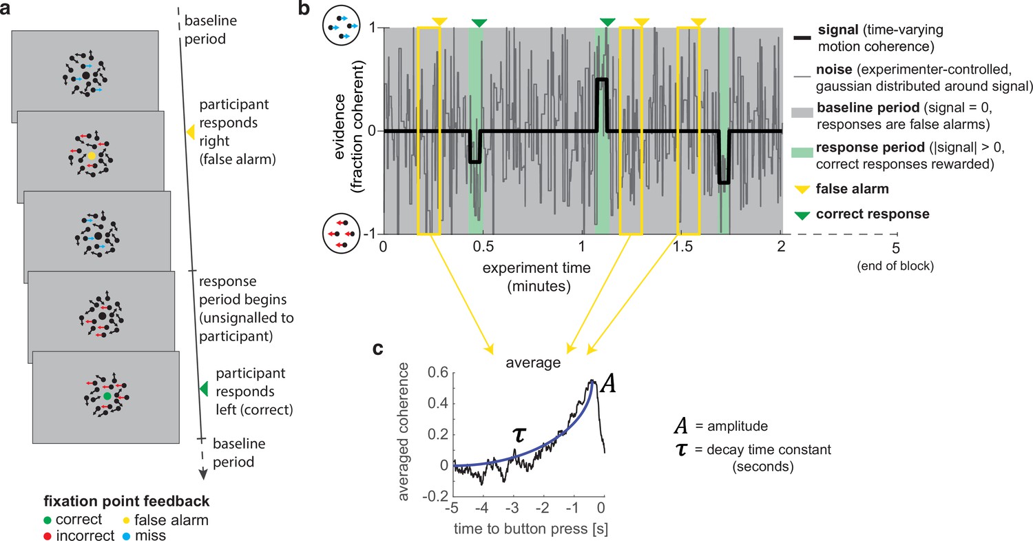
A novel, continuous version of the random dot kinematogram (RDK) paradigm allows empirical measurement of participants’ leaky evidence integration kernels in dynamic environments.
(a) Task design. Participants continuously attend to a centrally presented RDK stimulus, for 5 min at a time. They aim to successfully report motion direction during ‘response periods’ (when coherent motion signal is on average non-zero) and withhold responding during ‘baseline periods’ (when signal is on average zero). (b) Task structure (example block; response periods are ‘rare’). During both baseline (grey) and response periods (green), the signal (black line) is corrupted with experimenter-controlled noise (grey line). The noise fluctuations that precede each response (arrows) can be averaged to obtain the evidence integration kernel. (c) The resulting evidence integration kernel for false alarms is well described by an exponential decay function, whose decay time constant in seconds is controlled by the free parameter . The equation for this kernel is in the main text, and details of kernel fitting are provided in ‘Methods’.
Figure 2 with 1 supplement
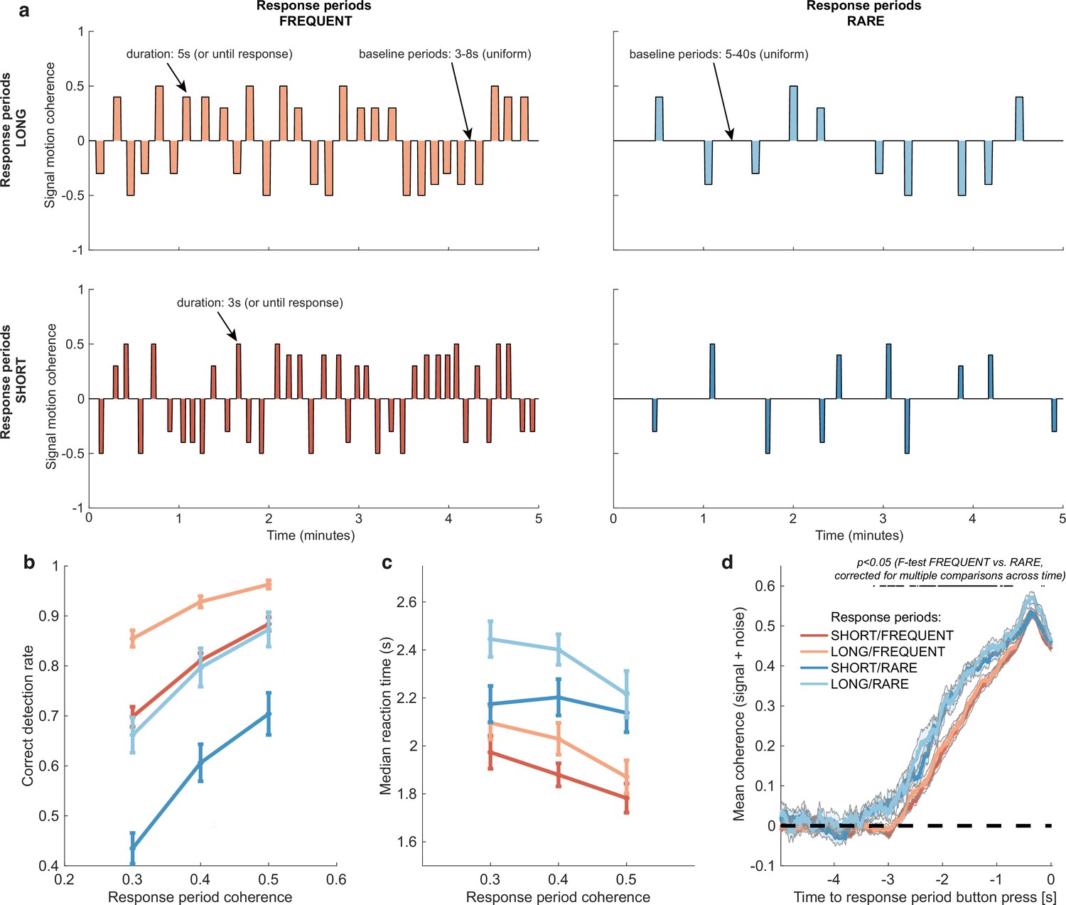
Variations in response period structure across different environments elicit behavioural adaptations in decision-making.
(a) Structure of response periods (signal only, before noise was added to the stimulus stream) across the different environments. This was manipulated in a 2 * 2 design, where response periods were either FREQUENT or RARE, and LONG or SHORT. Participants were extensively trained on these statistics prior to the task, and the current environment was explicitly cued to the participant. (b) Correct detection rate for all response periods. Participants successfully detected more response periods when they were LONG than SHORT (as would be expected, because the response period is longer), but also detected more when they were FREQUENT than RARE. (c) Median reaction time (time taken to respond after start of response period) for successfully reported response periods across the four conditions. Participants took longer in RARE versus FREQUENT conditions, and in LONG versus SHORT conditions. (d) Integration kernels for ‘response periods’ shows a main effect of FREQUENT versus RARE response periods, but unexpectedly no effect of LONG versus SHORT response periods. See main text for further discussion of this analysis. All plots in (b–d) show mean ± s.e. across 24 participants. Note that to make reaction times and integration kernels comparable between the four conditions, we only include those responses that were shorter than 3.5 s in analyses for (c) and (d) (i.e. the maximum response time in SHORT response periods).
Figure 2—figure supplement 1
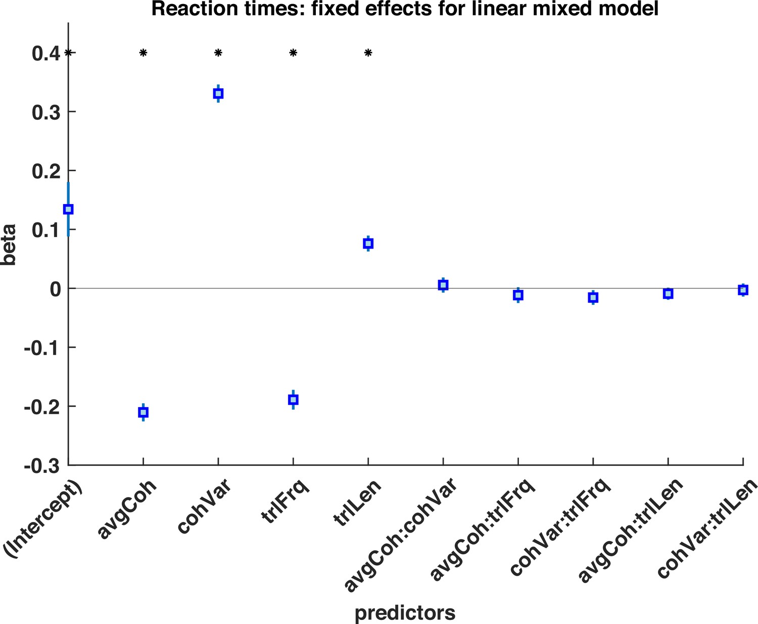
Logistic mixed model of subjects choices during response periods, with regressors of mean motion coherence (avgCoh), variance of motion coherence (cohVar), response period Frequency (trlFrq), response period length (trlLen), and interaction terms between these regressors.
The results indicate that both the mean motion coherence and variance of the motion coherence influenced participants’ choice, suggesting that participants used a strategy of detecting shifts in both mean and variance to detect response periods. * denotes p<0.05 significant effect across participants.
Figure 3 with 1 supplement
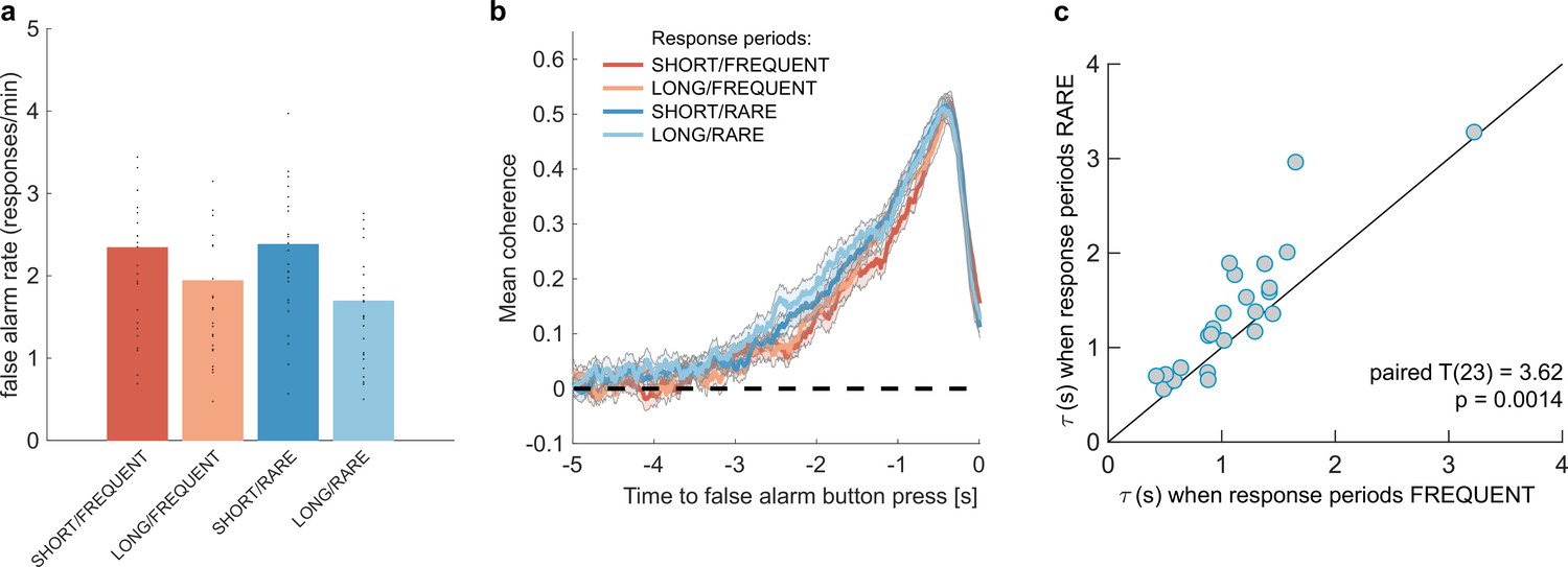
Changes in false alarm response frequency and evidence integration kernels across environments with different statistical structure.
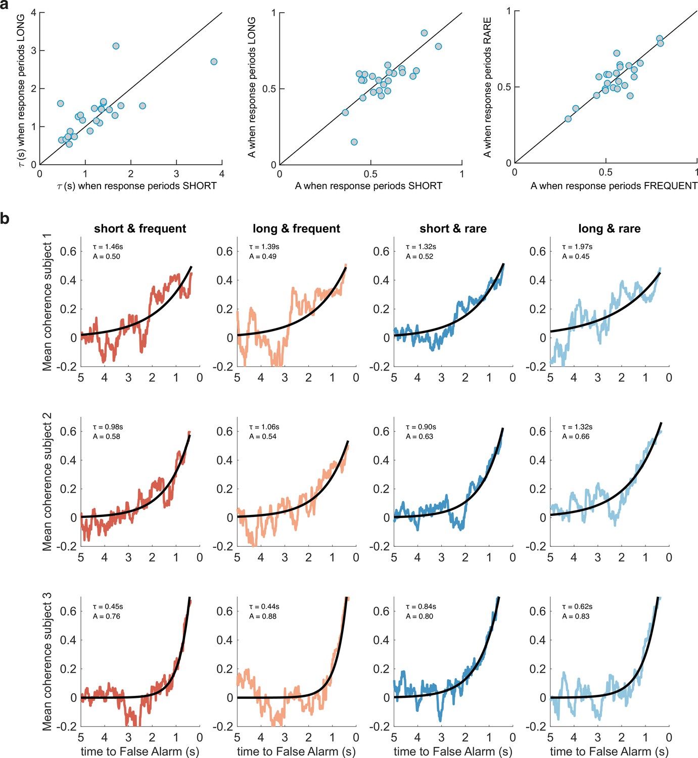
(a) False alarm rates (responses during baseline periods) showed a main effect of response period duration – participants showed significantly lower false alarm rates when response periods were LONG versus SHORT (F(1,23) = 58.67, p=8.98 * 10–8). This is consistent with having a more cautious response threshold (also evidenced by longer reaction times during response periods, see Figure 2c), although it could also be interpreted as shorter response periods inducing more confusion between signal and noise. (b) Integration kernels calculated for false alarms across the four conditions. Lines show mean +/- s.e. across 24 participants. (c) Exponential decay model fitted to individual participants’ kernels during false alarms shows a significantly longer decay time constant when response periods were RARE versus FREQUENT. The data points show the time constant, , for each participant after fitting a model of exponential decay to the integration kernel. The equation for this kernel is in the main text, and details of kernel fitting are provided in ‘Methods’.
Figure 3—figure supplement 1
Between-subject variability in evidence integration kernels exceeds between-condition variability.
(a) Left panel: unlike for RARE versus FREQUENT (Figure 3c), there was no significant difference in decay time constant for integration kernels for LONG versus SHORT. Similarly, there was no difference in amplitude parameter A for either of these comparisons (middle/right panels). (b) Variability across individuals, and comparative consistency across conditions, of integration kernels. This figure shows integration kernels from three example subjects in the experiment across the four conditions. Although our experiment primarily aimed to test whether integration kernels would be adapted to different environmental statistics (columns of figure), we found (unexpectedly) that different individuals had very different integration kernels (rows); some would integrate evidence over longer durations (e.g. top row), and others over far shorter durations (e.g. bottom row). All analyses are from false alarm responses only.
Figure 4 with 2 supplements
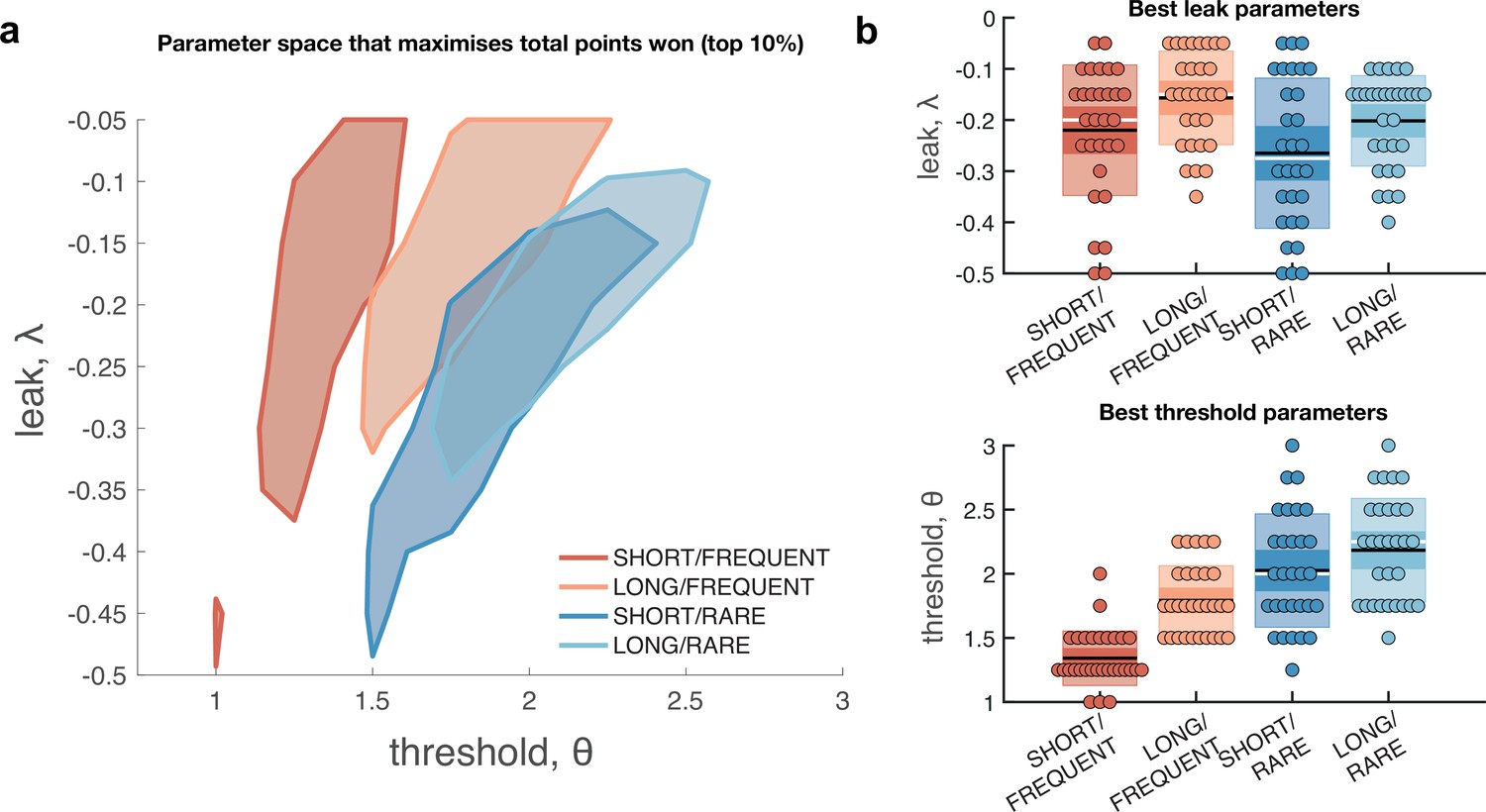
Optimal leak and threshold for a leaky accumulator model differs as a function of task condition.
(a) We performed a grid search over the parameters and θ to evaluate the performance (points won) for different parameterisations (Figure 4—figure supplement 1). The shaded area denotes the areas of model performance that lay in the top 10% of all models considered. The optimal area differs across conditions, and the optimal setting for leak and threshold co-vary with one another. (b) We used the evidence stream presented to each participant (each dot = one 5 min block), to identify the model parameterisation that would maximise total reward gained for each subject in each condition (see also Figure 4—figure supplement 2).
Figure 4—figure supplement 1
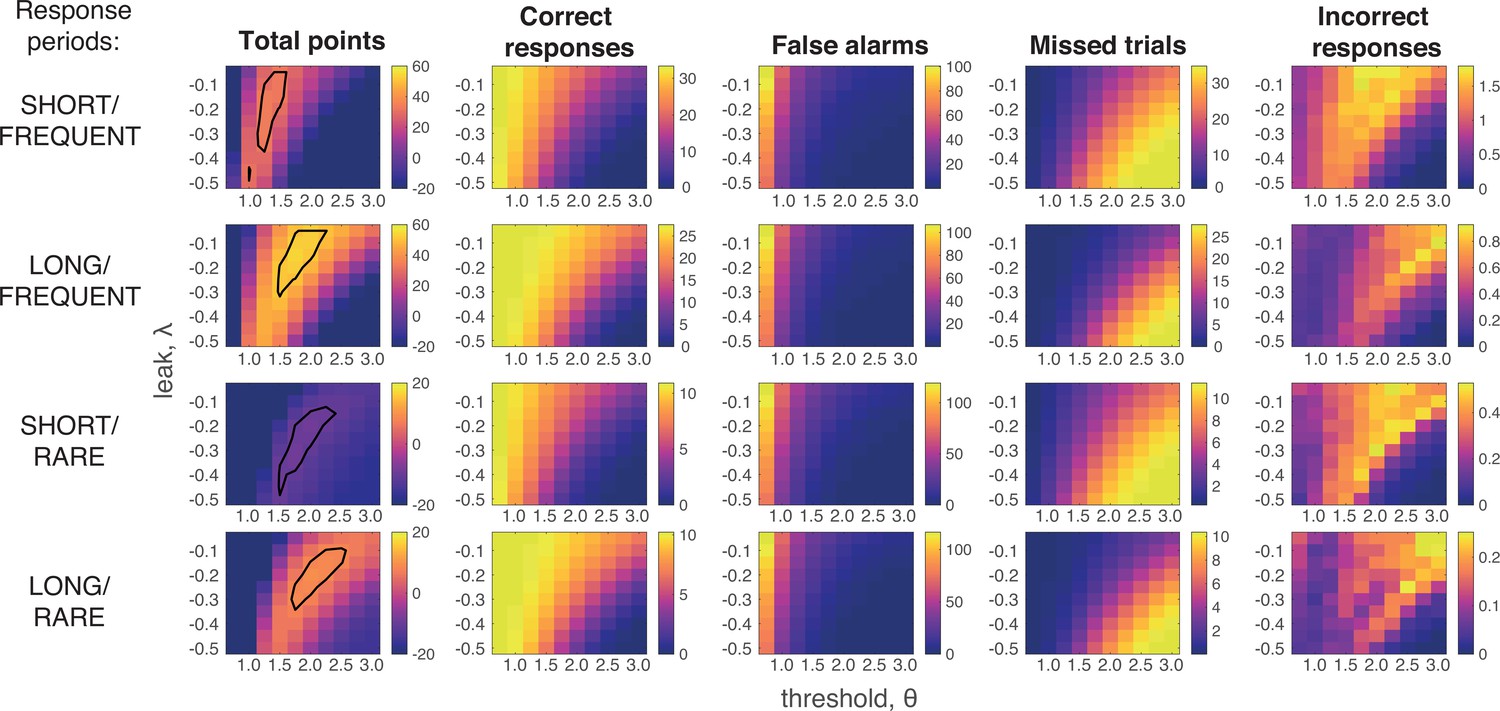
Grid search across parameter space for Ornstein–Uhlenbeck process.
We considered a plausible range of settings for the leak and threshold parameters that might maximise the total points won (left-hand column; top 10% of models enclosed in black line; see also main Figure 4a). The optimal model parameterisation depended upon a trade-off between the frequency of correct responses during response periods (second column) against the number of false alarms (third column) and missed trials (fourth column). As in human behaviour, the total number of ‘incorrect responses’ made (i.e. wrong response emitted during response window) were negligible.
Figure 4—figure supplement 2
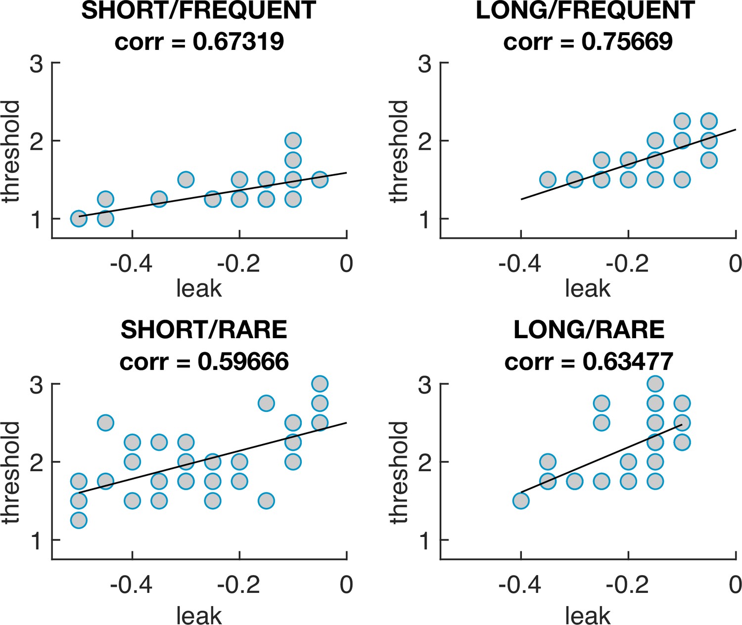
The optimal model parameters for leak and threshold correlate with each other.
The four graphs show the optimal model parameterisations for each individual subjects’ sensory evidence stream, for each of the four conditions (i.e. each dot = one 5 min stream of evidence, Figure 4b). In all four conditions, a model that is ‘less leaky’ (i.e. is closer to 0) is typically compensated by setting the decision threshold θ to be higher to achieve optimal performance (as also seen in Figure 4—figure supplement 1).
Figure 5
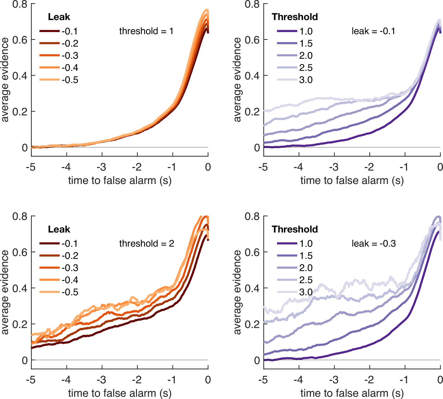
Variation in model threshold primarily determines decay time constant of integration kernels.
We performed an integration kernel analysis on false alarms emitted by the Ornstein–Uhlenbeck process with different settings for leak (λ, left column) and threshold (θ, right column) while holding the other parameter constant. Variation in θ would invariably affect the requirement for temporally sustained evidence to emit a false alarm (a higher threshold requiring sustained evidence); variation in primarily affect the amplitude of the eventual kernel.
Figure 6
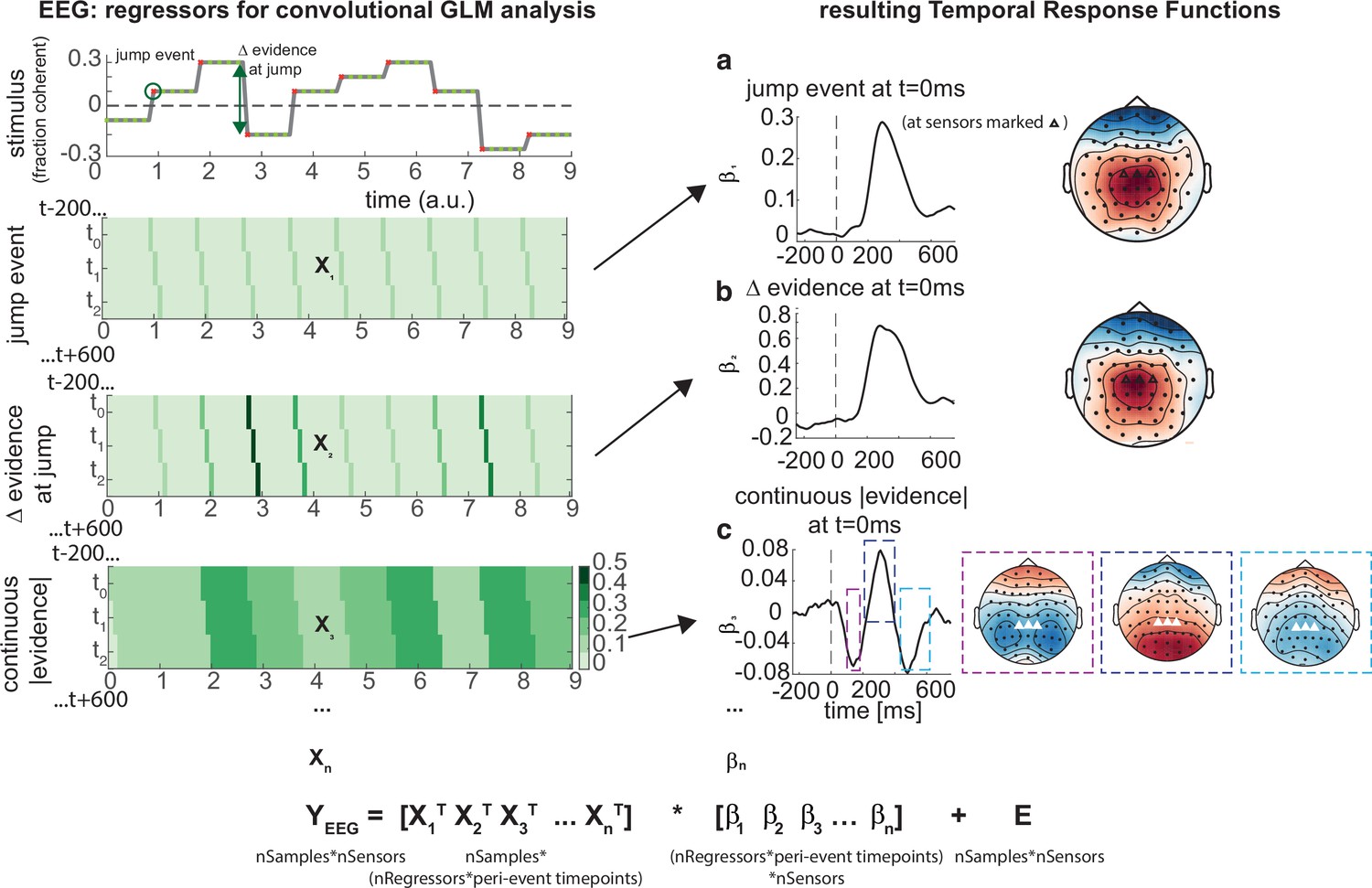
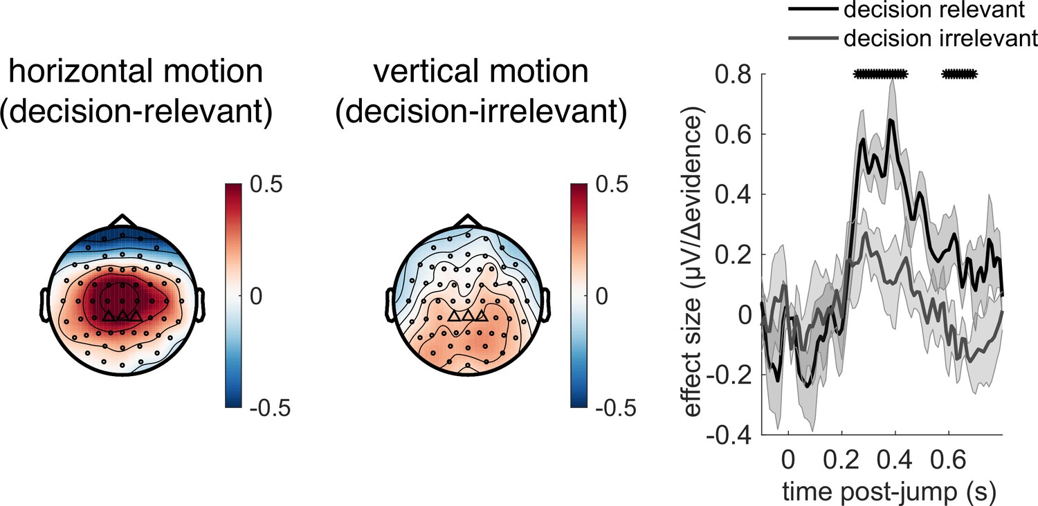
Deconvolutional general linear model to estimate electroencephalographic (EEG) temporal response functions to continuous, time-varying decision regressors.
The left-hand side of the figure shows an example evidence stream during the baseline period (note that inter-sample intervals are shown as fixed duration for clarity, rather than Poisson distributed as in the real experiment). Three example regressors are shown: (a) ‘jump event’, when there was a change in the noise coherence level; (b) '|Δ evidence|’, reflecting the magnitude of the jump update at each jump event; and (c) continuous |evidence|, reflecting the continuous absolute motion strength. For each of these regressors, a lagged version of the regressor timeseries is created to estimate the temporal response function (TRF) at each peri-event timepoint. This is then included in a large design matrix X, which is regressed onto continuous data Y at each sensor. This leads to a set of temporal response functions for each regressor at each sensor, shown on the right-hand side of the figure. The timecourse for each regressor shows the average regression weights at the three sensors highlighted with triangles on the scalp topography. Full details of the design matrix used in our analysis of the EEG data are provided in ‘Methods’.
Figure 7 with 2 supplements
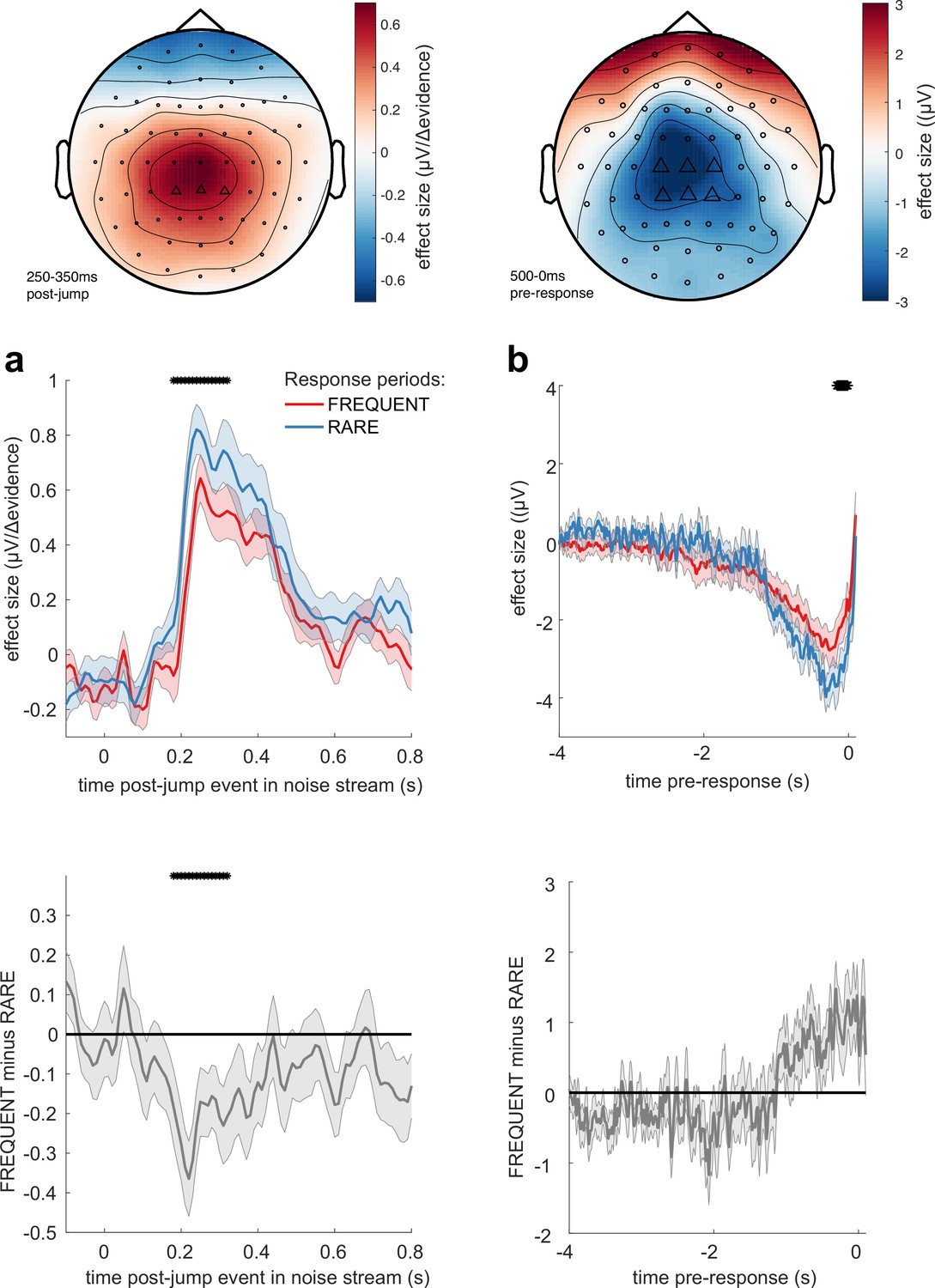
Adaptations of electroencephalographic (EEG) responses to sensory environments where response periods are RARE versus FREQUENT.
(a) Centroparietal electrodes (see triangles in scalp topography) showed a significantly greater response to Δevidence during ‘jump events’ in the noise stream when response periods were RARE than when they were FREQUENT. (b) Central and centroparietal electrodes showed a significantly greater negative-going potential immediately prior to a buttonpress during response periods. Lines and error bars show mean ± s.e.m. across 24 participants. * (solid black line at top of figure) denotes significant difference between FREQUENT and RARE (p<0.05, cluster corrected for multiple comparisons across time). Details of the permutation testing used for multiple-comparisons correction are provided in ‘Methods’.
Figure 7—figure supplement 1
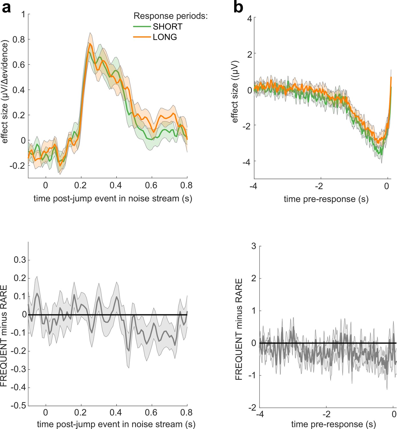
No significant differences in electroencephalographic (EEG) responses between conditions where response periods were SHORT versus LONG.
Figure 7—figure supplement 2
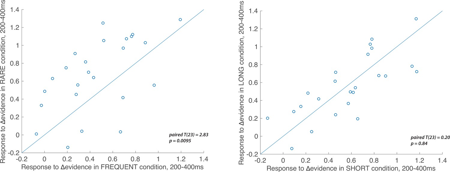
Individual subject electroencephalographic (EEG) effects for the Δevidence regressor over centroparietal electrodes from 200 to 400 ms after the change in evidence.
The left-hand panel shows the individual effects for the Δevidence regressor over centroparietal electrodes (see triangles in Figure 7), averaged within-participant for both FREQUENT and RARE conditions (each dot = 1 participant). The plot shows the significantly increased response to this regressor in RARE versus FREQUENT (T(23) = 2.83, p=0.0095). No such difference is seen for the equivalent plot comparing SHORT and LONG conditions (right-hand panel).
Figure 8
Control experiment demonstrates that response to |Δevidence| is primarily found to decision-relevant horizontal motion, but not decision-irrelevant vertical motion (with identical generative statistics).
Lines show mean +/- s.e.m. across 6 participants. * denotes timepoints where the response to |Δevidence| is significantly greater for decision-relevant motion than decision-irrelevant motion, while controlling for multiple-comparisons across time (see ‘Methods’).
Figure 9
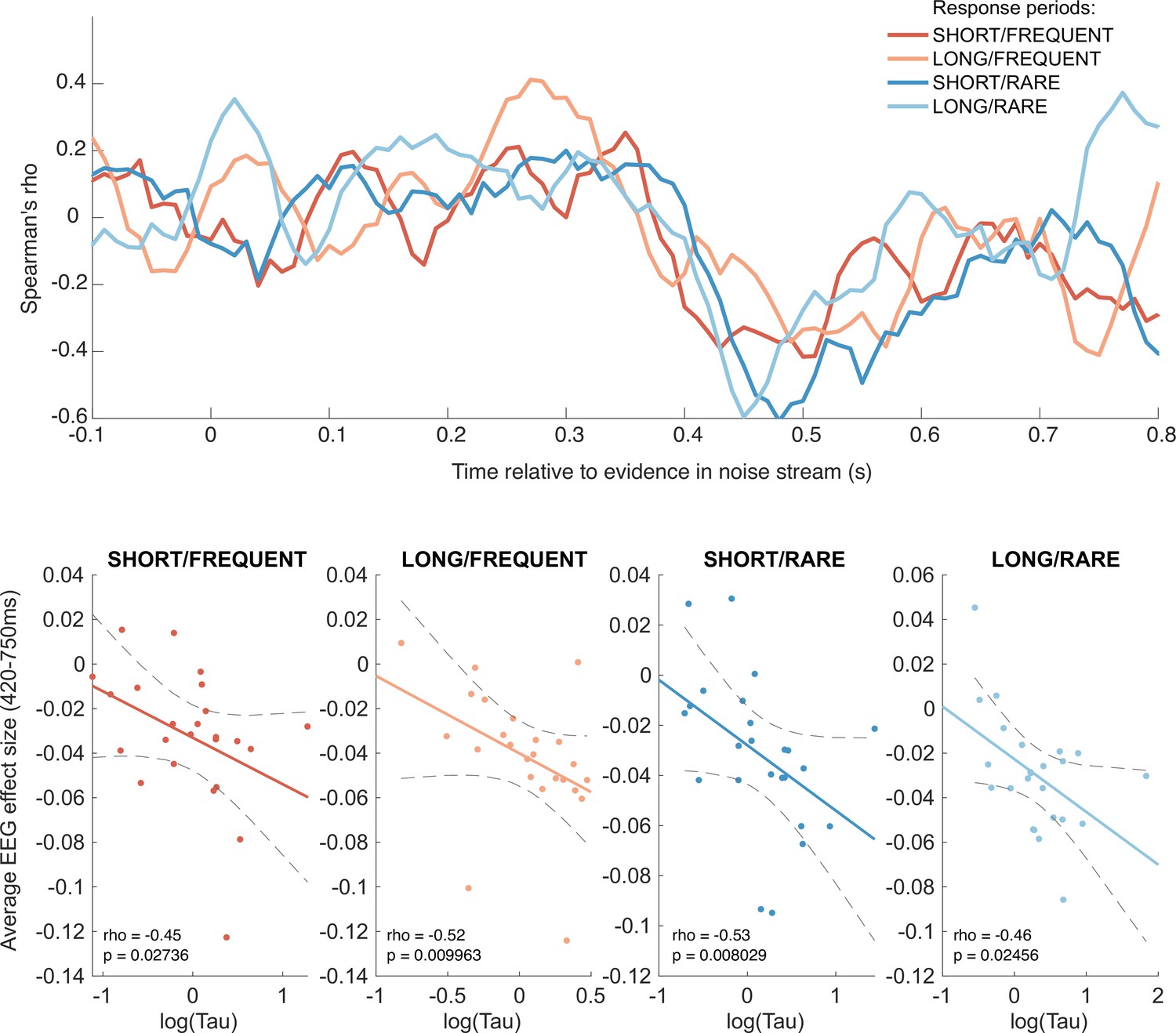
Behavioural-neural correlation (across subjects) of integration decay time constant and response to absolute sensory evidence in stimulus (see Figure 6c).
Top panel shows Spearman’s rank correlation between the time-varying electroencephalographic (EEG) beta for absolute sensory evidence and individual subjects’ parameter, separately for each of the four conditions. The negative-going correlation found in all four conditions from ~420 ms onwards coincides with the third, negative-going limb of the triphasic response to absolute sensory evidence shown in Figure 6c. Bottom panels show the correlation plotted separately for each of the four conditions. We plot the average EEG effect size against log() to allow for a straight-line fit (lines show mean ± 95% confidence intervals of a first-order polynomial fit between these two variables); we used Spearman’s rho to calculate the relationship, as it does not assume linearity.
Author response image 1

The average empirical standard deviation of the stimulus stream presented during each baseline period (‘baseline’) and response period (‘trial’), separated by each of the four conditions (F = frequent response periods, R = rare, L = long response periods, S = short).
Data were averaged across all response/baseline periods within the stimuli presented to each participant (each dot = 1 participant). Note that the standard deviation shown here is the standard deviation of motion coherence across frames of sensory evidence. This is smaller than the standard deviation of the generative distribution of ‘step’-changes in the motion coherence (std = 0.5 for baseline and 0.3 for response periods), because motion coherence remains constant for a period after each ‘step’ occurs.
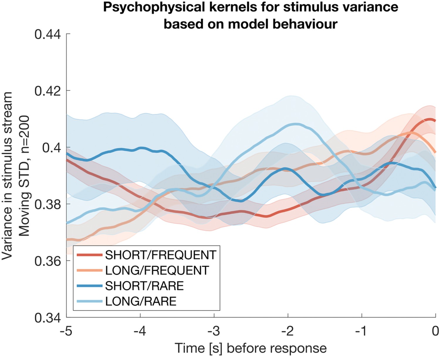
Author response image 2
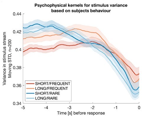
Integration kernels for stimulus variance, timelocked to false alarms made by participants in each of the four conditions.
Each line shows mean +/- s.e.m. (across participants) of the integration kernel for stimulus variance; in all four conditions, the reduction instimulus variance prior to a false alarm indicates that participants were likely performing stimulus detection in part using information about stimulus variance as well as stimulus mean (main Figures 2d, 3b).
Author response image 3
The same analysis as in Reviewer Response Figure 2, but now performed on simulated data from the Ornstein-Uhlenbeck model rather than participant behaviour.
The absence of any integration kernel confirms that the results in the previous figure are not artifactual.
Tables
Table 1
(Average) explained variance between regressors of the convolutional general linear model (GLM) for baseline periods.
Columns and rows are the different regressors used to investigate baseline periods. Between each pair of regressors for the key continuous variables, the explained variance (squared correlation coefficient) was calculated to ensure that these regressors were not correlated with each other prior to estimating the GLM.
| R2 | Jump | Jump level | Jump |Δevidence| | Continuous |evidence| |
|---|---|---|---|---|
| Jump | 1 | 0 | 0.01 | 0 |
| Jump level | 0 | 1 | 0.18 | 0.03 |
| Jump |Δevidence| | 0.01 | 0.18 | 1 | 0.01 |
| Continuous |evidence| | 0 | 0.03 | 0.01 | 1 |
Table 2
Design matrix.
This table describes the size of the design matrix assuming a sampling frequency of the electroencephalographic (EEG) signals of 100 Hz. For each regressor the number of lags pre- and post event and the total number of rows this regressor covers in the design matrix are described. The same number of lags was applied to vertical motion regressors for the control study.
| Regressor | Pre-event time in time-expanded design matrix (ms) | Post-event time in time-expanded design matrix (ms) | Total rows in the time-expanded design matrix |
|---|---|---|---|
| Jump event (stick function) | 1000 | 1500 | 251 |
| Jump level (|evidence| at each jump event) | 1000 | 1500 | 251 |
| Jump |Δevidence| (at each jump event) | 1500 | 1500 | 301 |
| Continuous |evidence| | 1500 | 1500 | 301 |
| Continuous (signed) evidence | 1500 | 1500 | 301 |
| Correct buttonpresses (stick function) | 5000 | 3500 | 851 |
| Correct buttonpresses (+1 for right, –1 for left) | 5000 | 3500 | 851 |
| False alarm buttonpresses (stick function) | 5000 | 3500 | 851 |
| False alarm buttonpresses (+1 for right, –1 for left) | 5000 | 3500 | 851 |
| Onset of response period (stick function) | 500 | 8000 | 851 |
| Response period |coherence| of response period (stick function) | 500 | 8000 | 851 |
Additional files
Download links
A two-part list of links to download the article, or parts of the article, in various formats.
Downloads (link to download the article as PDF)
Open citations (links to open the citations from this article in various online reference manager services)
Cite this article (links to download the citations from this article in formats compatible with various reference manager tools)
Quantifying decision-making in dynamic, continuously evolving environments
eLife 12:e82823.
https://doi.org/10.7554/eLife.82823


