Imaging analysis of six human histone H1 variants reveals universal enrichment of H1.2, H1.3, and H1.5 at the nuclear periphery and nucleolar H1X presence
- Molecular Biology Institute of Barcelona (IBMB-CSIC), Spain
Figures
Figure 1 with 1 supplement
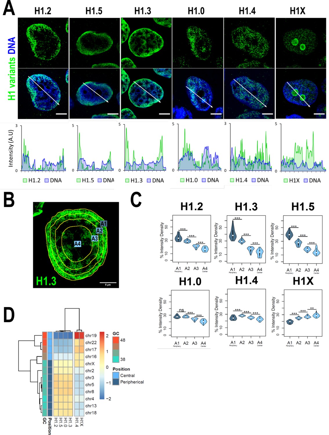
H1 variants are differentially enriched toward the nuclear periphery in T47D cells.
(A) Confocal immunofluorescence of H1 variants (green) and DNA staining (blue). Bottom panels show the intensity profiles of H1 variants and DNA along the arrows depicted in the upper panel. Scale bar: 5 µm. (B) Example of one cell stained with H1.3 antibody in which four sections of an equivalent area and convergent to the nuclear center are shown. Sections are named A1–A4, from the more peripheral section to the more central one. H1 variants immunofluorescence intensity was measured in each area and expressed as percentage. (C) Quantifications of H1 variants using the segmentation illustrated in (B), where n = 30 cells/condition were quantified, and data were represented in violin plots. Statistical differences between A1–A2, A2–A3, and A3–A4 for H1.0 and H1.4 are supported by paired t-test. (***) p-value <0.001; (**) p-value <0.01; (ns/non-significant) p-value >0.05. (D) H1 variants Input-subtracted ChIP-Seq median abundance per chromosome. Y-axis annotation indicated median %GC content per chromosome and their nuclear positions according to Boyle et al., 2001; Girelli et al., 2020.
Figure 1—figure supplement 1
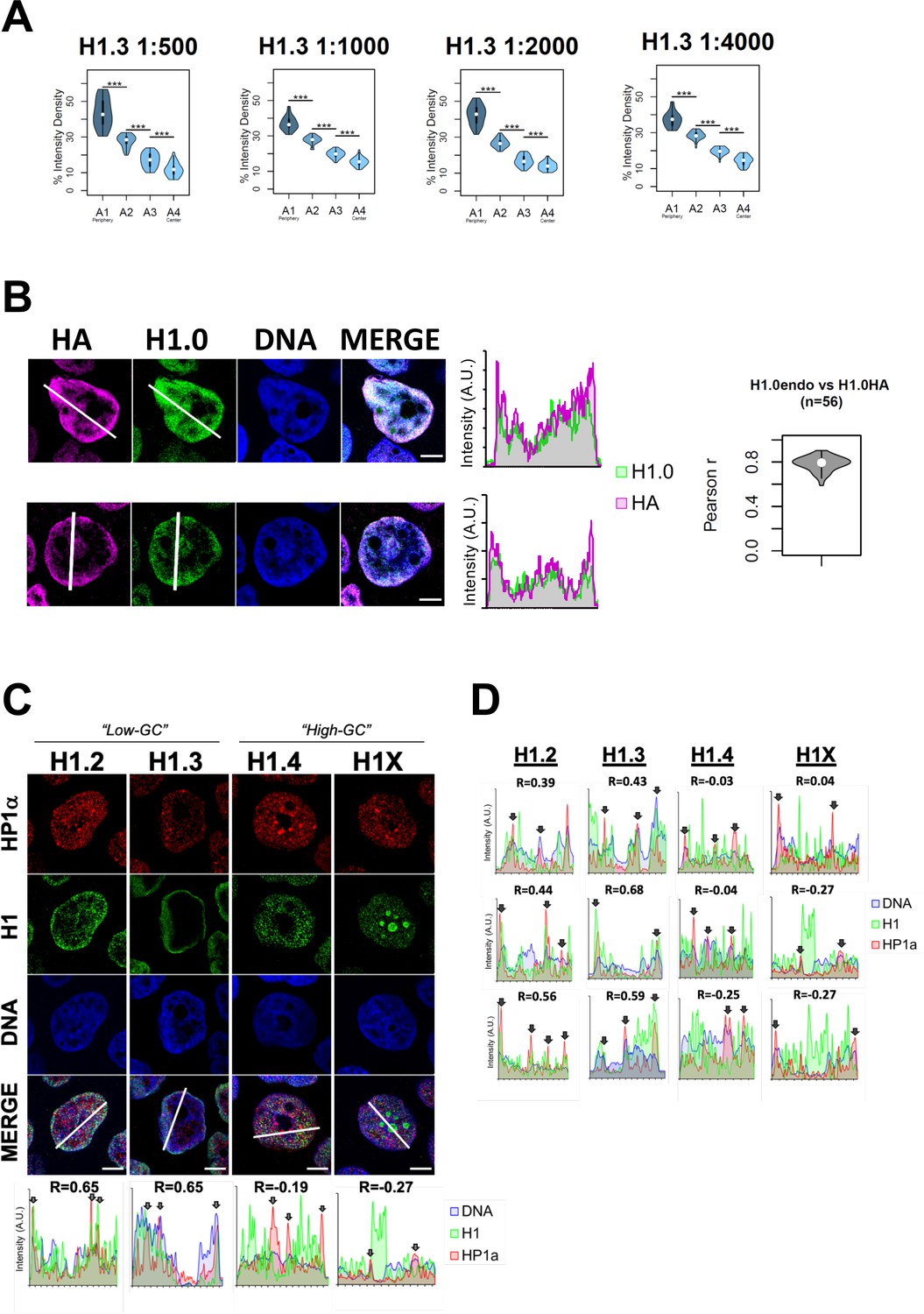
Endogenous H1 variants immunofluorescence controls and co-localization with heterochromatin protein HP1.
(A) To discard that the peripheral nuclear enrichment seen by immunofluorescence for some of the H1 variants is due to saturating antibody concentrations, we performed H1.3 immunofluorescence using serial dilutions of primary antibody. Graphs show immunofluorescence quantification signal of H1.3 using different antibody concentrations, as indicated. As illustrated in Figure 1B, four sections of an equivalent area and convergent to the nuclear center are created per each cell. Sections are named A1–A4, from the more peripheral section to the more central one. H1.3 immunofluorescence intensity is measured in each area and expressed as percentage. n = 30 cells/condition were quantified, and data were represented in violin plots. Statistical differences between consecutive sections are supported by paired t-test. (***) p-value <0.001. Of note, a clear peripheral distribution was observed for H1.3 despite the antibody concentration used. (B) Immunofluorescence of T47D cells stably expressing HA-tagged H1.0 was done using H1.0 and HA antibodies to evaluate co-localization between both antibodies signals. Panels show intensity profiles of H1.0 and HA antibodies along the arrows depicted. Scale bar: 5 µm. A violin plot showing the Pearson correlation between H1.0 and HA signals in n = 56 cells is included. The high overlap and correlation obtained between HA and H1.0 prove the ability of the antibody to recognize epitopes in different chromatin environments despite H1 location. They also prove that the nuclear peripheral enrichment observed for some variants is not due to the inaccessibility of the antibody to more central or occluded regions. (C) Confocal immunofluorescence of HP1alpha (red), H1 variants (green), and DNA staining (blue). Bottom panels show the intensity profiles along the white lines depicted in the merge panel. Correlation between HP1a and the corresponding H1 variant along the depicted line is indicated above the graphs. In the bottom profiles, gray arrows point to HP1a foci. Scale bar: 5 µm. In (D), three additional profiles per H1 variant are shown.
Figure 2 with 3 supplements
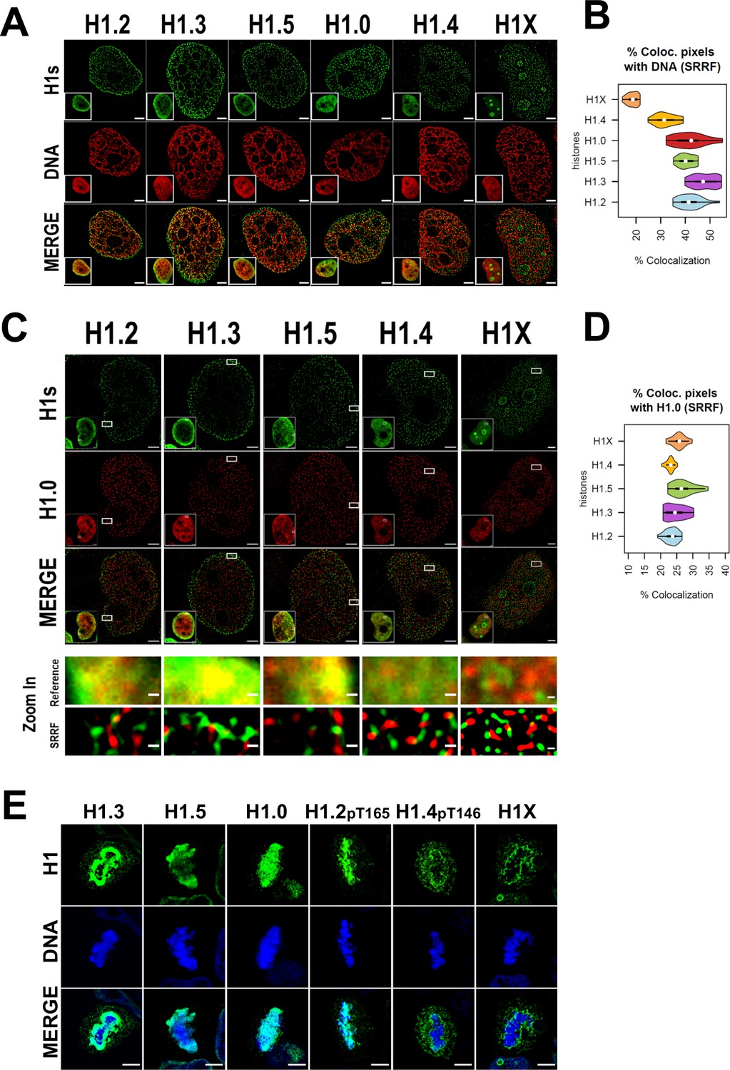
Super-resolution imaging shows that H1 variants occupy different regions in single cells.
(A) Super-resolution radial fluctuation (SRRF) images of H1 variants (green) and DNA (red). Bottom-left: Insets show the Reference confocal image in each case. Scale bar: 2 µm. (B) Percentage of co-localized pixels between H1 variants and DNA by SRRF imaging. n = 20 cells/condition were quantified and values distribution were represented as violin plots. (C) SRRF images of H1 variants (green) and H1.0 (red). Bottom-left: Insets show the Reference confocal image in each case. In the bottom panel, the highlighted zoom-in insets at confocal (reference) or SRRF resolutions are shown. Scale bar: 2 µm, scale bar in zoom-in insets: 200 nm. (D) Percentage of co-localized pixels of H1 variants with H1.0 by SRRF imaging. n = 20 cells/condition were quantified and values distribution were represented as violin plots. (E) Immunofluorescence of H1 variants (green) and DNA (blue) during metaphase. As H1.2 and H1.4 signal was not detected during metaphase (see main text and Figure 2—figure supplements 2 and 3), antibodies recognizing specific phosphorylations of these variants were used. To see H1 variants profiles along mitosis progression, see Figure 2—figure supplements 2 and 3. Scale bar: 5 µm.
Figure 2—figure supplement 1
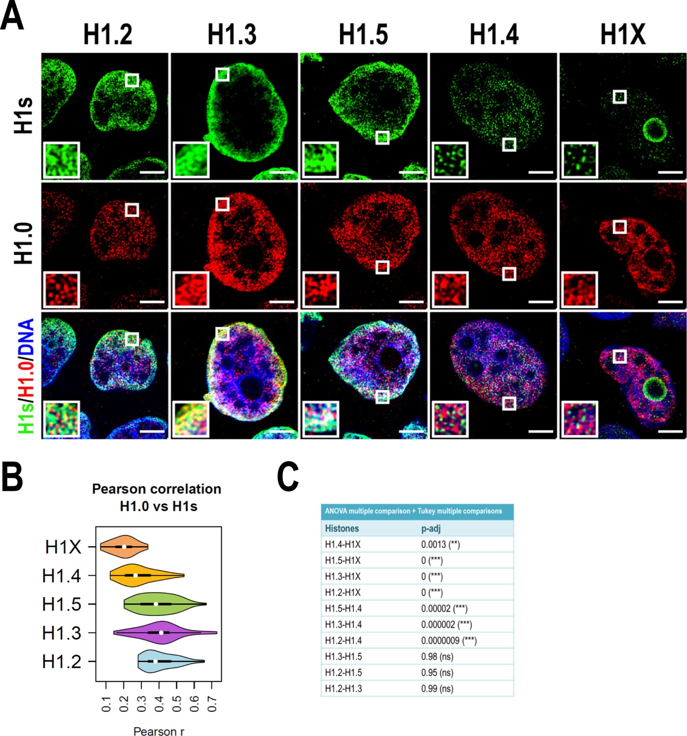
H1 variants co-localization at confocal resolution.
(A) Confocal immunofluorescence of the indicated H1 variants (green) with H1.0 (red) and DNA staining (blue). Zoom-in insets highlight H1.0-peripheral enrichment territories. Scale bar: 5 µm. (B) Violin plots showing the Pearson correlation coefficient (r) distribution of H1 variants with H1.0 in n = 40 cells/condition. (C) Statistical comparison of results shown in (B). Analysis of variance (ANOVA) multiple comparison test revealed that significant differences exist between groups. Tukey multiple comparison test was used to compare the H1s-H1.0 r values distribution between different H1s. p-adjusted values are shown (***) p-adj <0.001; (**) p-adj <0.01; (ns/non-significant) (p-adj >0.05).
Figure 2—figure supplement 2
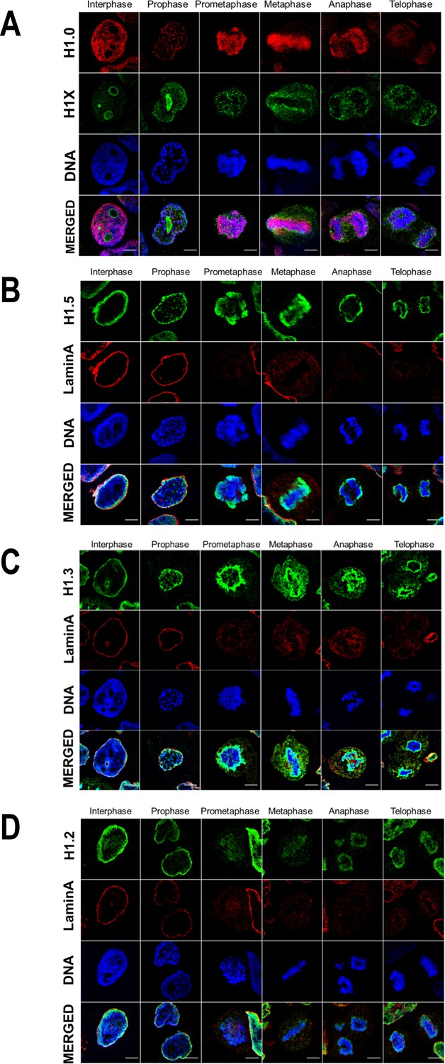
H1 variants distribution patterns along mitosis phases.
Immunofluorescence of H1 variants and LaminA along the distinct mitotic phases. In all cases, DNA staining is also shown. (A) Replication-independent H1.0 and H1X variants. (B) H1.5 and Lamin A. (C) H1.3 and Lamin A. (D) H1.2 and Lamin A. Scale bar: 5 µm.
Figure 2—figure supplement 3
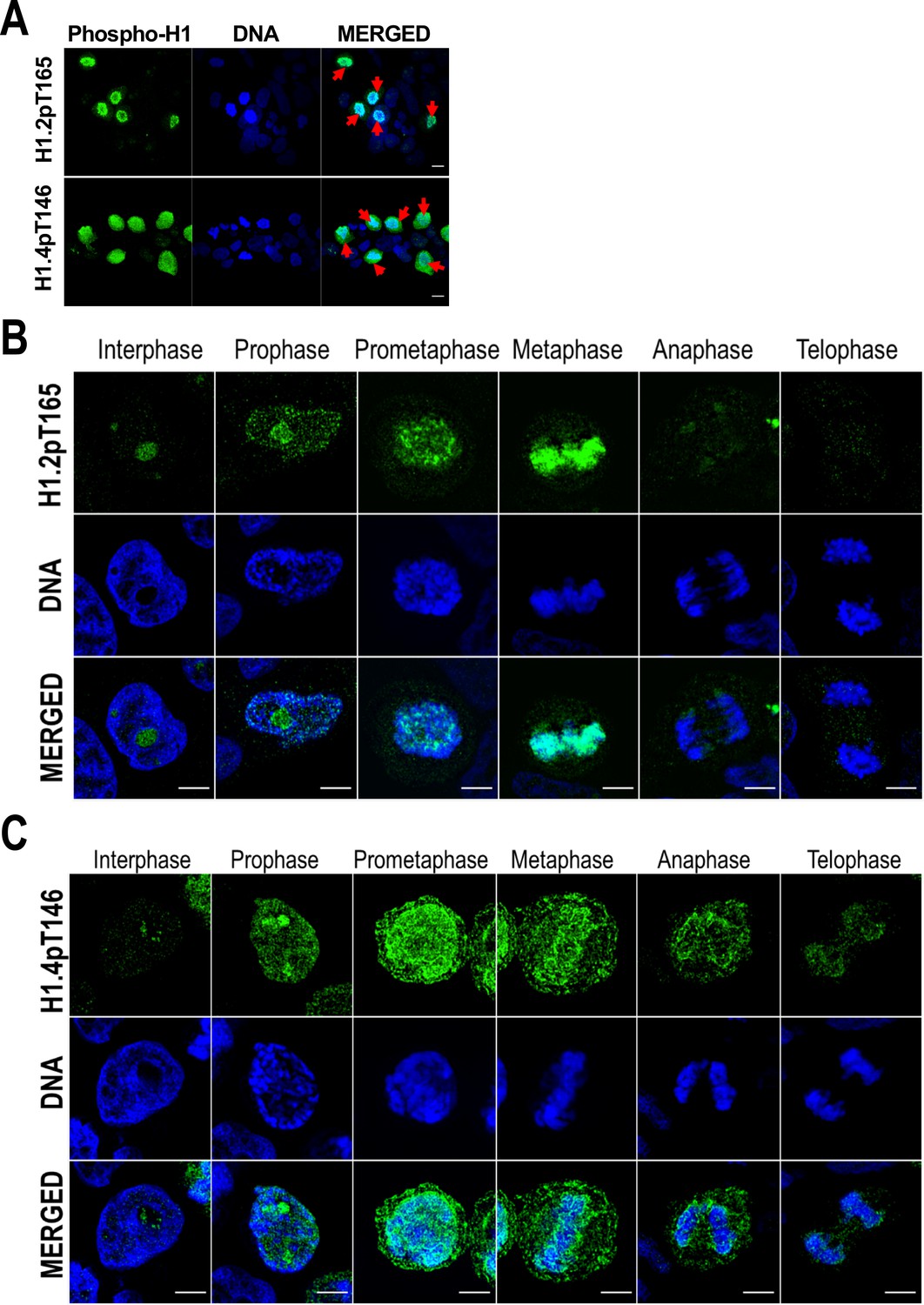
H1 variants phosphorylation during mitosis.
(A) Immunofluorescence of H1.2-pT165 and H1.4pT146. A Z-stack maximum projection is shown. Mitotic cells are marked by a red arrow. Scale bar: 10 µm. Immunofluorescence of phosphorylated H1.2-pT165 (B) and H1.4-pT146 (C) along the distinct mitotic phases. DNA staining is also shown. Scale bar: 5 µm.
Figure 3 with 1 supplement
H1 variants presence within lamina-associated domains (LADs) and nucleoli.
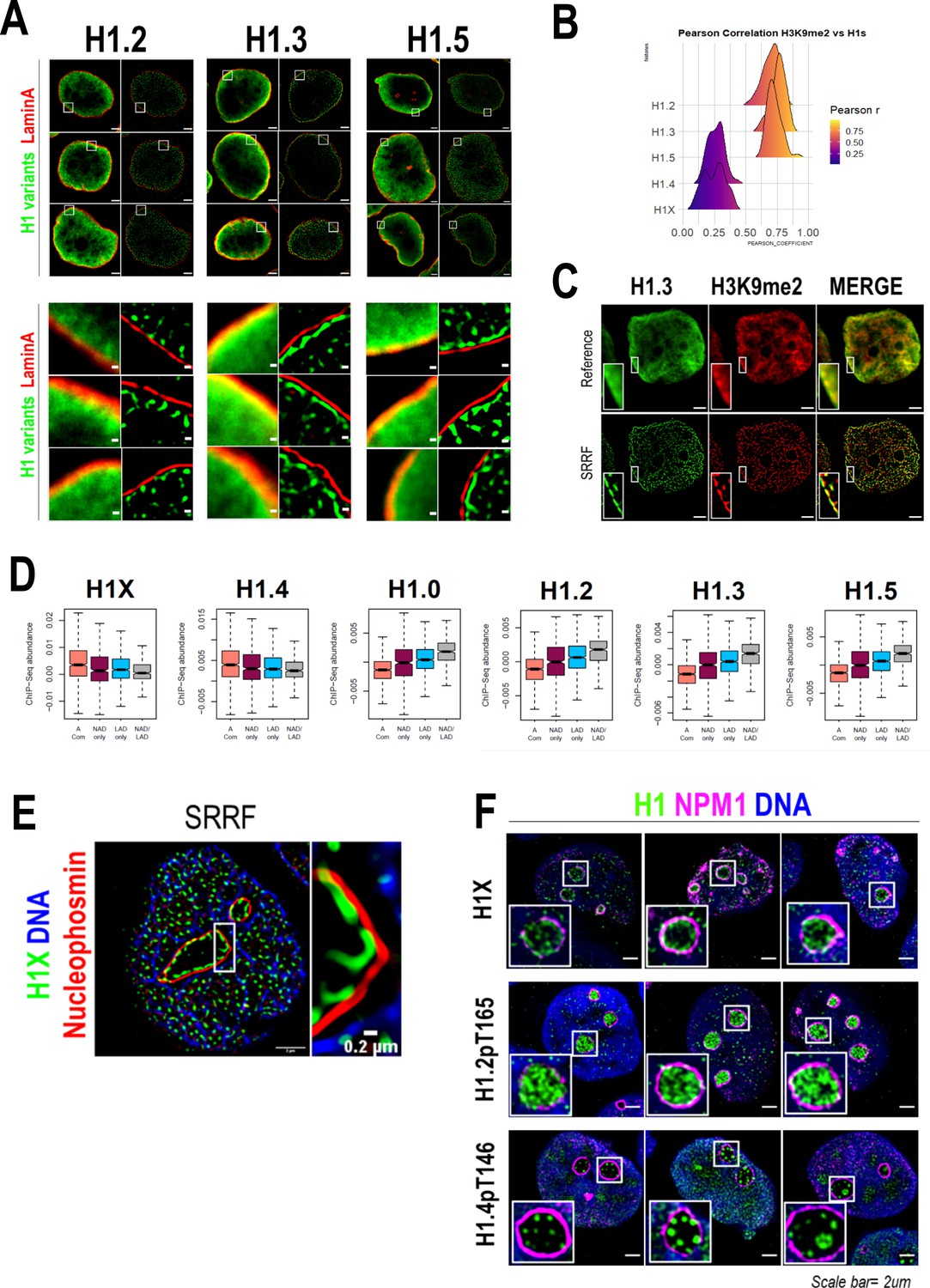
(A) Confocal (left) and super-resolution (right) images of a T47D cells stained for H1.2, H1.3, or H1.5 (in green) and Lamin A (in red) obtained using SRRF. Full nuclei (upper panel) and zoomed views of nuclear periphery (bottom panel) are shown. Scale bars: 2 µm (upper panel) and 200 nm (bottom panel). Three representative cells are shown for each H1 variant. (B) Pearson correlation coefficient (r) of H1 variants and H3K9me2 co-immunostaining signal. r values distribution in n = 50 cells/condition are shown. Representative immunofluorescence images of H1 variants and H3K9me2 are shown in Figure 3—figure supplement 1A. Scale bar: 5 µm. (C) H1.3 and H3K9me2 immunofluorescence at confocal (reference) and super-resolution (SRRF) level. A zoom-in inset of the peripheral layer formed by both H1.3 and H3K9me3 is shown. Scaler bar: 2 µm. (D) Boxplots show the Input-subtracted H1 variants ChIP-Seq abundance within regions exclusively defined as nucleolus-associated domains (NADs) (NAD only) or LADs (LAD only) and those genomic segments defined as both NADs and LADs (NAD/LAD). A compartment regions are included as a reference. NADs coordinates were extracted from Peng et al., 2023. (E) Representative SRRF image of H1X, NPM1, and DNA. Zoom-in highlights the H1X nucleolar layer. Scale bar: 2 µm. Scale bar in zoom-in: 0.2 µm. (F) Immunofluorescence of H1X, H1.2-pT165, or H1.4-pT146, Nucleophosmin (NPM1) and DNA. Insets show a zoom-in of a single nucleolus. Scale bar: 2 µm. Three representative cells are shown for each H1.
Figure 3—figure supplement 1
H1 variants within lamina-associated domains (LADs) and nucleoli under basal and upon ribosomal DNA (rDNA) transcription inhibition.
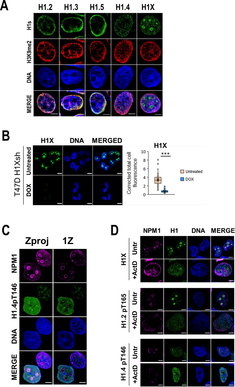
(A) Representative confocal immunofluorescence images of H1 variants (green), H3K9me2 (red), and DNA (blue). (B) Immunofluorescence of H1X and DNA in T47D H1Xsh −/+ Dox. A Z-stack of five consecutive Z planes is shown. Scale bar: 10 µm. H1X immunofluorescence signal quantification (n = 41 cells/condition) is shown and supported by paired t-test. (***) p-value <0.001. (C) Immunofluorescence of Nucleophosmin (NPM1), H1.4-pT146, and DNA in T47D cells. A unique central confocal Z plane (1Z) or the Z maximum projection (Zproj) are shown. Scale bar: 5 µm. (D) Immunofluorescence of H1X, H1.2p-T165, or H1.4-pT146 (green) co-immunostained with Nucleophosmin (magenta) and DNA (blue) under Untreated or Act-D-treated conditions. Scale bar: 5 µm.
Figure 4 with 1 supplement
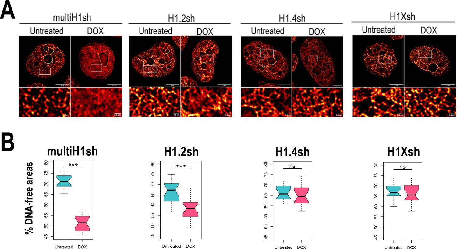
Chromatin structural changes upon H1 depletion.
(A) Representative super-resolution radial fluctuation (SRRF) images of DNA staining in the different H1 knock-downs (KD) conditions indicated (multi-H1, H1.2, H1.4, and H1X Dox-inducible shRNAs). In the bottom panels, a zoom-in inset is shown to appreciate DNA pattern in both Untreated and Dox conditions. Scale bar: 5 µm (full nucleus) and 500 nm (zoom-in). (B) DNA-free areas percentage quantification in the different H1 KDs. n = 20 cells/condition were quantified and the boxplot were constructed with the 20 average values in each condition. Statistical differences between Untreated and Dox-treated conditions are supported by paired t-test. (***) p-value <0.001; (ns/non-significant) p-value >0.05. Additional representative images and full quantification are shown in Figure 4—figure supplement 1.
Figure 4—figure supplement 1
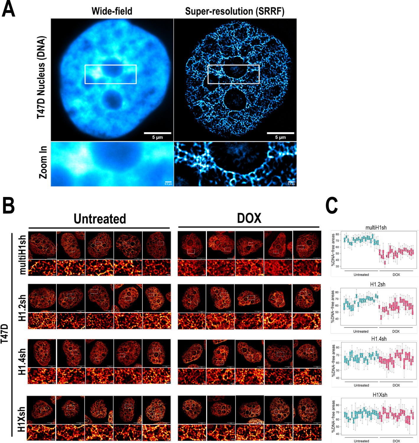
Super-resolution imaging of DNA upon different H1 knock-downs (KD) conditions.
(A) Representative images of DNA staining visualized with wide-field or super-resolution (SRRF) microscopy in a T47D nucleus. Bottom panels show a zoom-in of the perinucleolar region. Scale bar: 5 µm (full nucleus) or 500 nm (zoom-in insets). (B) Additional representative SRRF images of DNA staining in the different H1 KD conditions (multi-H1, H1.2, H1.4, and H1X Dox-inducible shRNAs). In the bottom pannels, a zoom-in inset is shown to appreciate DNA pattern in both Untreated and Dox conditions. Scale bar: 5 µm (full nucleus) and 500 nm (zoom-in). (C) Quantification of % DNA-free areas within n = 20 cells per condition.
Figure 5 with 5 supplements
Nuclear distribution of H1 variants across multiple human cell lines.
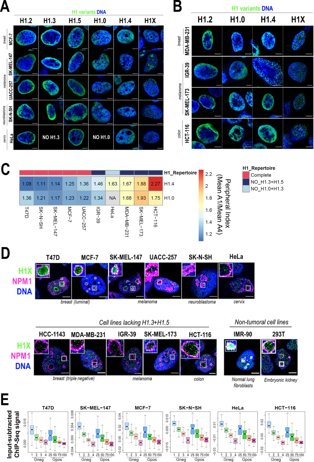
(A) Immunofluorescence analysis of H1 variants (green) with DNA staining (blue) in different cancer cell lines. Merged images are shown. H1.3 and H1.0 grids in HeLa cells are empty, as HeLa cells do not express these variants. Tumoral origin of the cell lines is indicated. Scale bar: 5 µm. (B) Immunofluorescence analysis of H1 variants (green) with DNA staining (blue) in cell lines lacking H1.3 and H1.5. Merged images are shown. Tumoral origin of the cell lines is indicated. Scale bar: 5 µm. (C) H1.4 and H1.0 show a more peripheral distribution in cell lines with a compromised H1 repertoire. Numbers correspond to peripheral index value in each cell line and color coded as indicated. Each nucleus was divided into four equivalent sections A1–A4 and immunofluorescence signal of H1.4 or H1.0 was quantified. Peripheral index was defined as the ratio between average value in A1 peripheral section and A4 central section. (D) Immunofluorescence of H1X (green), nucleolar marker Nucleophosmin (NPM1; magenta), and DNA staining (blue). Merged images are shown. Insets show a zoom-in of a single nucleolus. Bottom panel includes cell lines lacking H1.3 and H1.5. Cell line origin is indicated. Scale bar: 5 µm. (E) Boxplots show the H1X Input-subtracted ChIP-Seq signal at eight groups of Giemsa bands in six different cancer cell lines. G-bands groups were defined according to Serna-Pujol et al., 2021 (see Materials and methods).
Figure 5—figure supplement 1
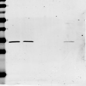
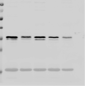
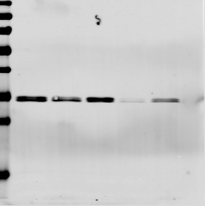
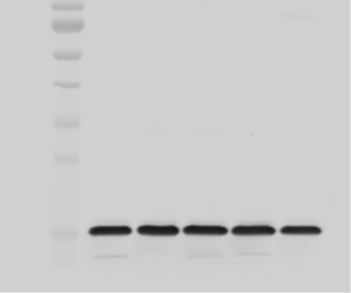
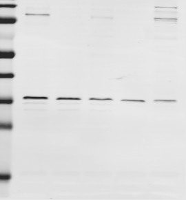
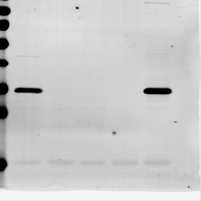
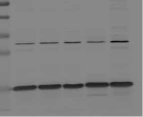
H1 protein and mRNA complement across cell lines.
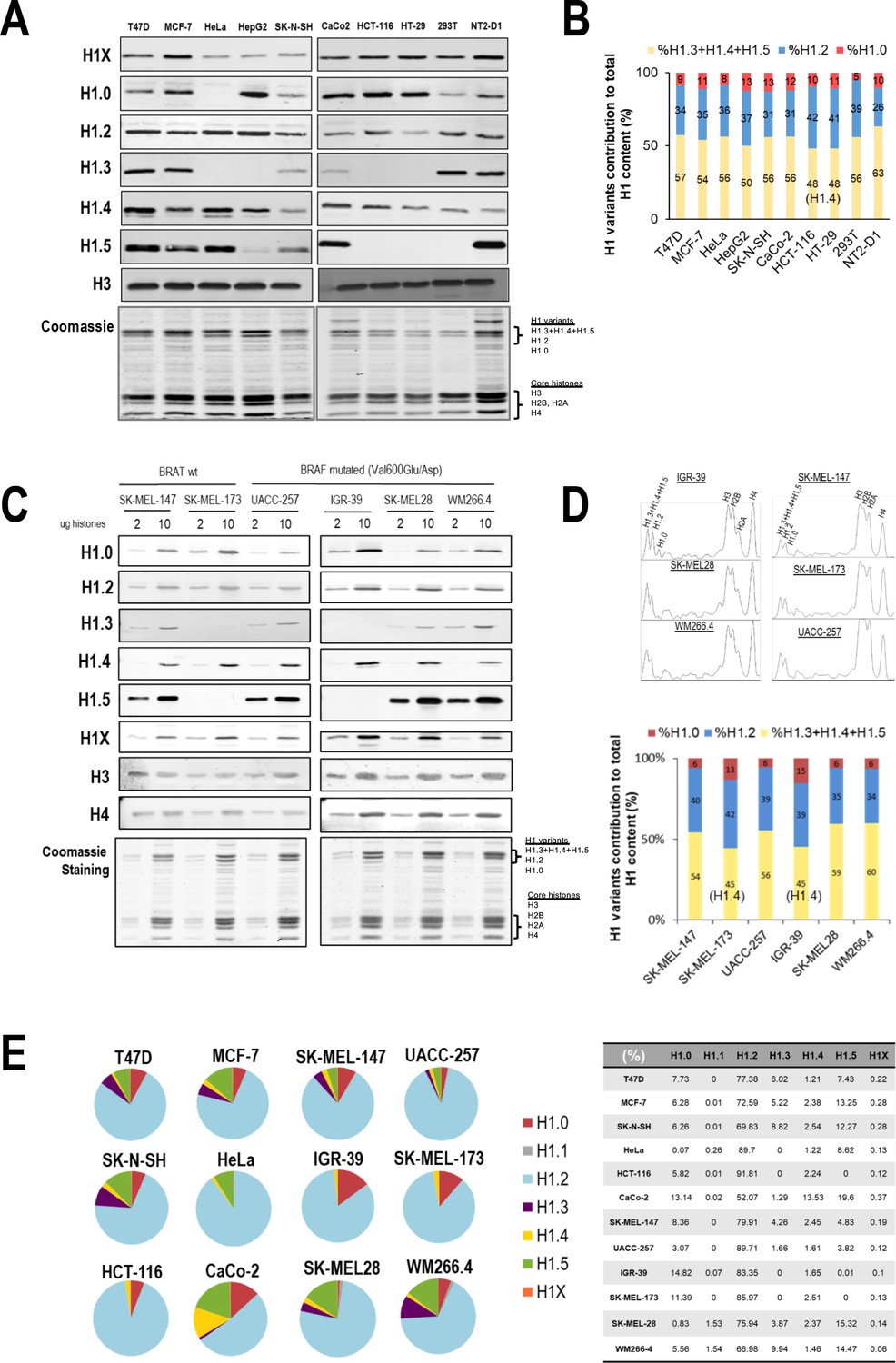
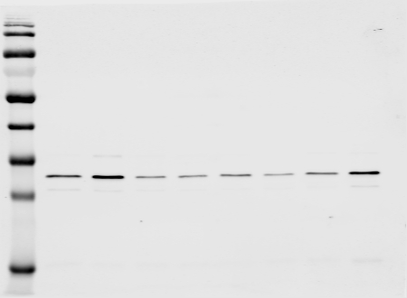
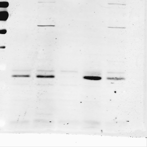
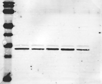
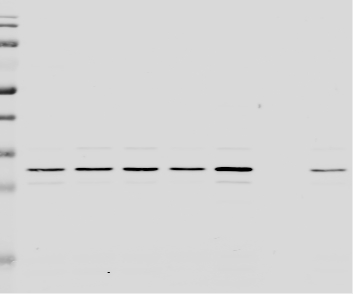
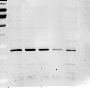
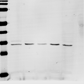
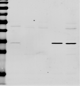
(A) Immunoblot analysis of H1 variants in histones extracts from different tumoral and non-tumoral cell lines. Histone H3 is added as a nuclear control and Coomassie staining is shown. (B) Coomassie staining quantification of histone extracts from cell lines shown in (A). Graph shows the contribution of the three H1 Coomassie bands to total H1 content. Data are normalized by H4 band and represented as percentage. (C) Immunoblot of H1 variants in histones extracts (2 or 10 µg) from six melanoma cell lines. Histone H3 and H4 are added as nuclear controls and Coomassie staining is shown. BRAF mutation status is indicated. (D) Top panels show the ImageJ profiling of histones Coomassie shown in (C). The bottom panel represents the contribution of the three H1 Coomassie bands to total H1 content. Data are normalized by H4 band and represented as percentage. In cell lines lacking H1.3 and H1.5, the upper H1 Coomassie band corresponds to H1.4. (E) Gene expression levels of H1 variants in different cancer cell lines were analyzed by reverse-transcriptase-quantitative PCR (RT-qPCR). Data are corrected by GAPDH and normalized by the corresponding genomic DNA amplification. Corrected expression data from all H1 variants are summed to calculate total H1 expression and represent values as percentage. Data are represented as pie charts or numerically collected in a table.
-
Figure 5—figure supplement 1—source data 1
PDF containing original scans of the relevant Western blot analysis shown in Figure 5—figure supplement 1A, C with highlighted bands.
- https://cdn.elifesciences.org/articles/91306/elife-91306-fig5-figsupp1-data1-v1.pdf
-
Figure 5—figure supplement 1—source data 2
Original file for the Western blot analysis in Figure 5—figure supplement 1A, left panels (H1X).
- https://cdn.elifesciences.org/articles/91306/elife-91306-fig5-figsupp1-data2-v1.jpg
-
Figure 5—figure supplement 1—source data 3
Original file for the Western blot analysis in Figure 5—figure supplement 1A, left panels (H1.0).
- https://cdn.elifesciences.org/articles/91306/elife-91306-fig5-figsupp1-data3-v1.jpg
-
Figure 5—figure supplement 1—source data 4
Original file for the Western blot analysis in Figure 5—figure supplement 1A, left panels (H1.2).
- https://cdn.elifesciences.org/articles/91306/elife-91306-fig5-figsupp1-data4-v1.jpg
-
Figure 5—figure supplement 1—source data 5
Original file for the Western blot analysis in Figure 5—figure supplement 1A, left panels (H1.3).
- https://cdn.elifesciences.org/articles/91306/elife-91306-fig5-figsupp1-data5-v1.jpg
-
Figure 5—figure supplement 1—source data 6
Original file for the Western blot analysis in Figure 5—figure supplement 1A, left panels (H1.4).
- https://cdn.elifesciences.org/articles/91306/elife-91306-fig5-figsupp1-data6-v1.jpg
-
Figure 5—figure supplement 1—source data 7
Original file for the Western blot analysis in Figure 5—figure supplement 1A, left panels (H1.5).
- https://cdn.elifesciences.org/articles/91306/elife-91306-fig5-figsupp1-data7-v1.jpg
-
Figure 5—figure supplement 1—source data 8
Original file for the Western blot analysis in Figure 5—figure supplement 1A, left panels (H3).
- https://cdn.elifesciences.org/articles/91306/elife-91306-fig5-figsupp1-data8-v1.jpg
-
Figure 5—figure supplement 1—source data 9
Original file for the Western blot analysis in Figure 5—figure supplement 1A, right panels (H1X).
- https://cdn.elifesciences.org/articles/91306/elife-91306-fig5-figsupp1-data9-v1.jpg
-
Figure 5—figure supplement 1—source data 10
Original file for the Western blot analysis in Figure 5—figure supplement 1A, right panels (H1.0).
- https://cdn.elifesciences.org/articles/91306/elife-91306-fig5-figsupp1-data10-v1.jpg
-
Figure 5—figure supplement 1—source data 11
Original file for the Western blot analysis in Figure 5—figure supplement 1A, right panels (H1.2).
- https://cdn.elifesciences.org/articles/91306/elife-91306-fig5-figsupp1-data11-v1.jpg
-
Figure 5—figure supplement 1—source data 12
Original file for the Western blot analysis in Figure 5—figure supplement 1A, right panels (H1.3).
- https://cdn.elifesciences.org/articles/91306/elife-91306-fig5-figsupp1-data12-v1.jpg
-
Figure 5—figure supplement 1—source data 13
Original file for the Western blot analysis in Figure 5—figure supplement 1A, right panels (H1.4).
- https://cdn.elifesciences.org/articles/91306/elife-91306-fig5-figsupp1-data13-v1.jpg
-
Figure 5—figure supplement 1—source data 14
Original file for the Western blot analysis in Figure 5—figure supplement 1A, right panels (H1.5).
- https://cdn.elifesciences.org/articles/91306/elife-91306-fig5-figsupp1-data14-v1.jpg
-
Figure 5—figure supplement 1—source data 15
Original file for the Western blot analysis in Figure 5—figure supplement 1A, right panels (H3).
- https://cdn.elifesciences.org/articles/91306/elife-91306-fig5-figsupp1-data15-v1.jpg
-
Figure 5—figure supplement 1—source data 16
Original file for the Western blot analysis in Figure 5—figure supplement 1C, left panels (H1X).
- https://cdn.elifesciences.org/articles/91306/elife-91306-fig5-figsupp1-data16-v1.tif
-
Figure 5—figure supplement 1—source data 17
Original file for the Western blot analysis in Figure 5—figure supplement 1C, left panels (H1.0).
- https://cdn.elifesciences.org/articles/91306/elife-91306-fig5-figsupp1-data17-v1.tif
-
Figure 5—figure supplement 1—source data 18
Original file for the Western blot analysis in Figure 5—figure supplement 1C, left panels (H1.2).
- https://cdn.elifesciences.org/articles/91306/elife-91306-fig5-figsupp1-data18-v1.tif
-
Figure 5—figure supplement 1—source data 19
Original file for the Western blot analysis in Figure 5—figure supplement 1C, left panels (H1.3).
- https://cdn.elifesciences.org/articles/91306/elife-91306-fig5-figsupp1-data19-v1.tif
-
Figure 5—figure supplement 1—source data 20
Original file for the Western blot analysis in Figure 5—figure supplement 1C, left panels (H1.4).
- https://cdn.elifesciences.org/articles/91306/elife-91306-fig5-figsupp1-data20-v1.tif
-
Figure 5—figure supplement 1—source data 21
Original file for the Western blot analysis in Figure 5—figure supplement 1C, left panels (H1.5).
- https://cdn.elifesciences.org/articles/91306/elife-91306-fig5-figsupp1-data21-v1.tif
-
Figure 5—figure supplement 1—source data 22
Original file for the Western blot analysis in Figure 5—figure supplement 1C, left panels (H3).
- https://cdn.elifesciences.org/articles/91306/elife-91306-fig5-figsupp1-data22-v1.tif
-
Figure 5—figure supplement 1—source data 23
Original file for the Western blot analysis in Figure 5—figure supplement 1C, left panels (H4).
- https://cdn.elifesciences.org/articles/91306/elife-91306-fig5-figsupp1-data23-v1.tif
-
Figure 5—figure supplement 1—source data 24
Original file for the Western blot analysis in Figure 5—figure supplement 1C, right panels (H1X).
- https://cdn.elifesciences.org/articles/91306/elife-91306-fig5-figsupp1-data24-v1.tif
-
Figure 5—figure supplement 1—source data 25
Original file for the Western blot analysis in Figure 5—figure supplement 1C, right panels (H1.0).
- https://cdn.elifesciences.org/articles/91306/elife-91306-fig5-figsupp1-data25-v1.tif
-
Figure 5—figure supplement 1—source data 26
Original file for the Western blot analysis in Figure 5—figure supplement 1C right panels (H1.2).
- https://cdn.elifesciences.org/articles/91306/elife-91306-fig5-figsupp1-data26-v1.tif
-
Figure 5—figure supplement 1—source data 27
Original file for the Western blot analysis in Figure 5—figure supplement 1C, right panels (H1.3).
- https://cdn.elifesciences.org/articles/91306/elife-91306-fig5-figsupp1-data27-v1.tif
-
Figure 5—figure supplement 1—source data 28
Original file for the Western blot analysis in Figure 5—figure supplement 1C, right panels (H1.4).
- https://cdn.elifesciences.org/articles/91306/elife-91306-fig5-figsupp1-data28-v1.tif
-
Figure 5—figure supplement 1—source data 29
Original file for the Western blot analysis in Figure 5—figure supplement 1C, right panels (H1.5).
- https://cdn.elifesciences.org/articles/91306/elife-91306-fig5-figsupp1-data29-v1.tif
-
Figure 5—figure supplement 1—source data 30
Original file for the Western blot analysis in Figure 5—figure supplement 1C, right panels (H3).
- https://cdn.elifesciences.org/articles/91306/elife-91306-fig5-figsupp1-data30-v1.tif
-
Figure 5—figure supplement 1—source data 31
Original file for the Western blot analysis in Figure 5—figure supplement 1C, right panels (H4).
- https://cdn.elifesciences.org/articles/91306/elife-91306-fig5-figsupp1-data31-v1.tif
Figure 5—figure supplement 2
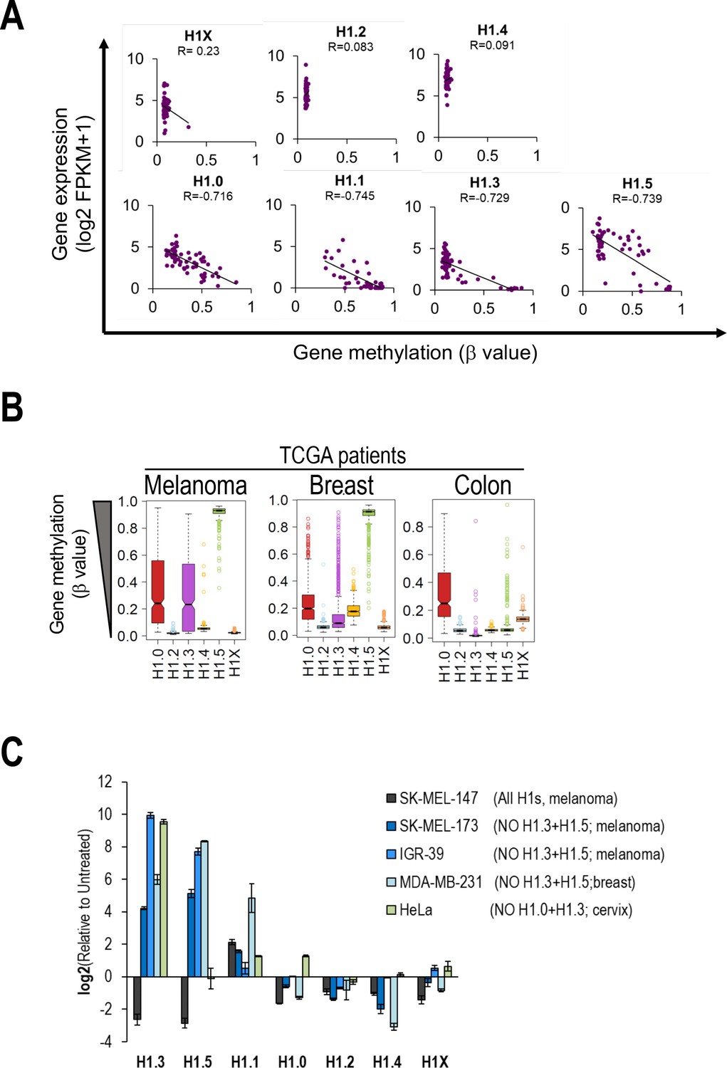
H1 variants expression regulation by DNA methylation.
(A) Scatterplots between H1 variants expression (Y-axis) and H1 gene methylation (X-axis) from NCI-60 public data. Gene expression from total RNA-Seq data is expressed in log2(FPKM + 1) while gene methylation is expressed as b value (β = 0 is totally unmethylated and β = 1 is totally methylated). Each dot represents a cell line from the NCI-60 panel. Pearson correlation coefficients (R) are shown. (B) Boxplots show the DNA methylation of H1 genes in different cancer datasets from The Cancer Genome Atlas (TCGA) project. Gene methylation is expressed as β value (β = 0 is totally unmethylated and β = 1 is totally methylated). (C) H1 variants expression levels in different cell lines under Untreated and aza-treated conditions were analyzed by reverse-transcriptase-quantitative PCR (RT-qPCR). Barplot shows relative expression of H1 variants upon aza treatment compared to Untreated condition, corrected by GAPDH and expressed as log2. SK-MEL-147 is added as a control cell line which expresses all H1 variants (except H1.1).
Figure 5—figure supplement 3
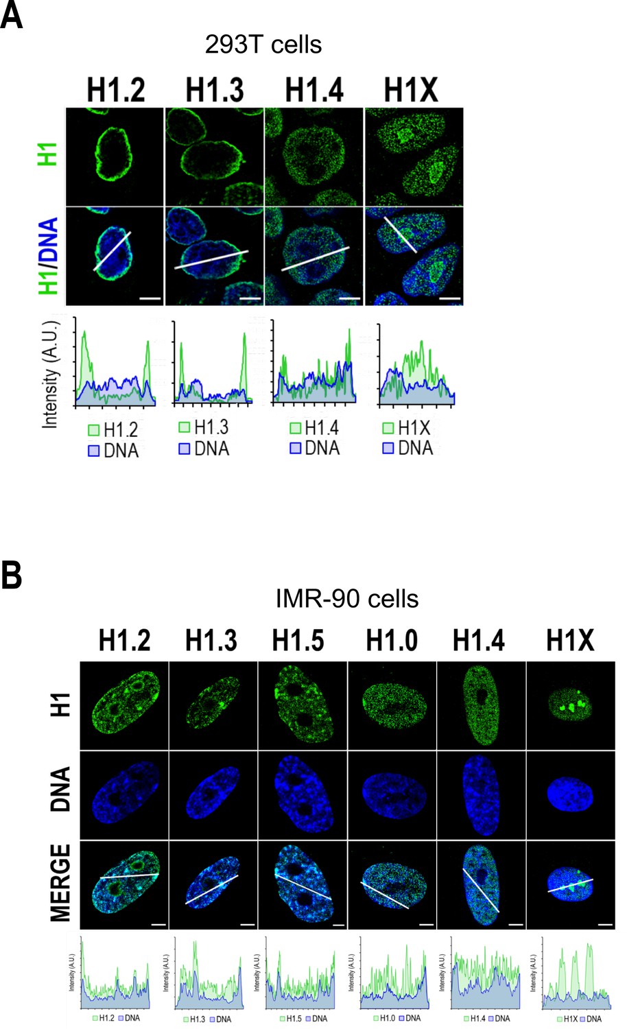
H1 variants nuclear distribution in non-tumoral cell lines.
Confocal immunofluorescence of H1 variants (green) and DNA staining (blue) in 293T (A) or IMR-90 (B) cells. Bottom panels show the intensity profiles of H1 variants and DNA along the arrows depicted in the corresponding upper panel. Scale bar: 5 µm. Of note, 293T do not express H1.5 and have very low levels of H1.0 (see Figure 5—figure supplement 1A). Indeed, most 293T cells are H1.0-negative in immunofluorescence. Regarding IMR-90 cells (B), it is important to note that these cells have a characteristic DNA staining pattern with DNA foci. H1.2, H1.3, H1.5, and H1.0 variants are highly enriched in these DNA foci, including those in the periphery. Thus, these profiles support the enrichment of these variants at heterochromatin or low-GC regions, present, but not limited to the nuclear periphery. On the contrary, H1.4 and H1X are distributed throughout the whole nucleus, with H1X being highly present at nucleoli, but they are not enriched in these heterochromatic foci. This observation supports the two H1 groups, in terms of distribution, observed in T47D.
Figure 5—figure supplement 4
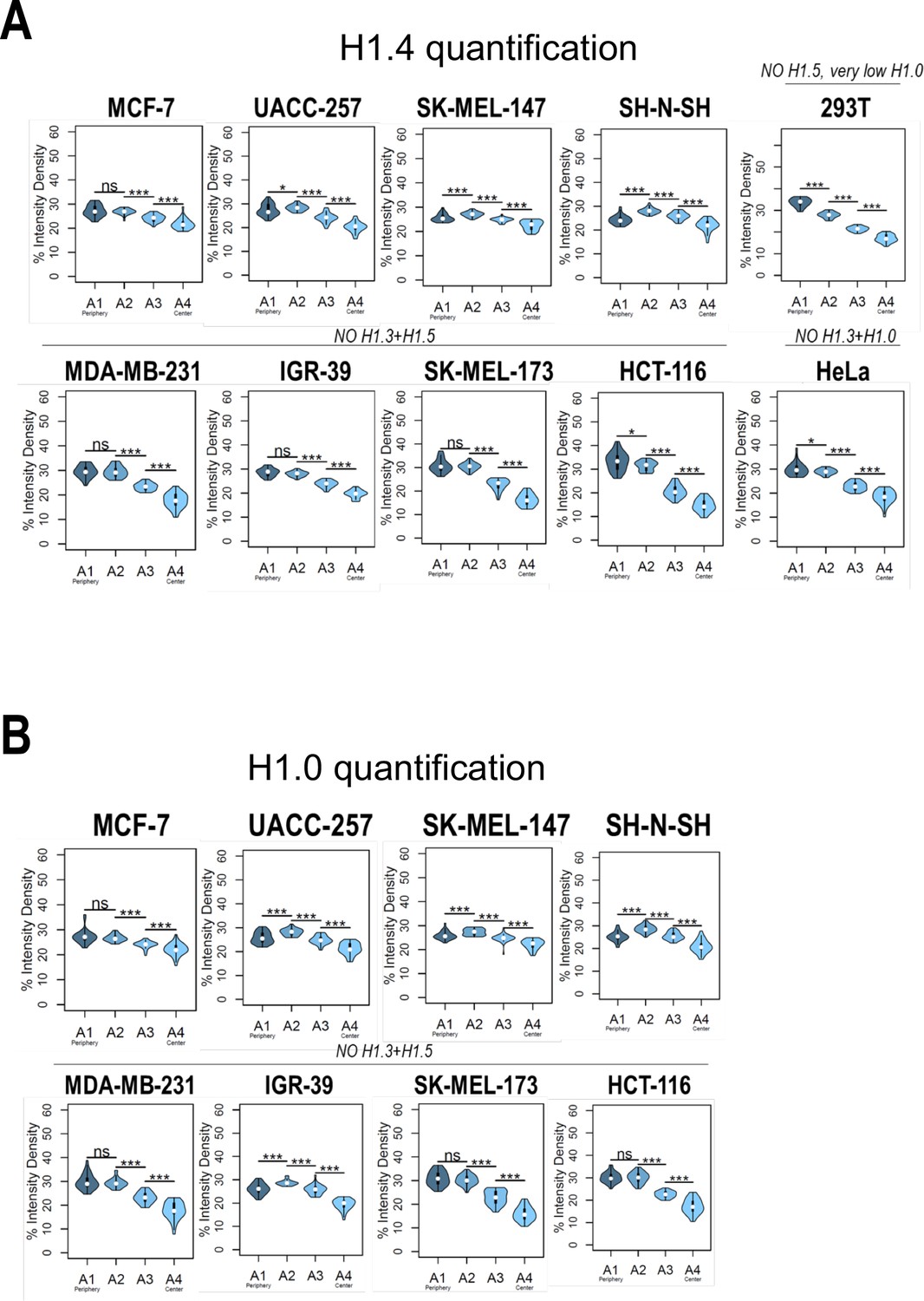
Nuclear radial distribution of H1.4 and H1.0 across cell lines.
Graphs show immunofluorescence quantification signal of (A) H1.4 and (B) H1.0 in different cell lines. As illustrated in Figure 1B, four sections of an equivalent area and convergent to the nuclear center are created per each cell. Sections are named A1–A4, from the more peripheral section to the more central one. H1 variants immunofluorescence intensity is measured in each area and expressed as percentage. Cell lines with a compromised H1 somatic repertoire are indicated. n = 30 cells/cell line were quantified, and data were represented in violin plots. Statistical differences between A1–A2, A2–A3, and A3–A4 are supported by paired t-test. (***) p-value <0,001; (*) p-value <0.05; (ns/non-significant) p-value >0.05.
Figure 5—figure supplement 5
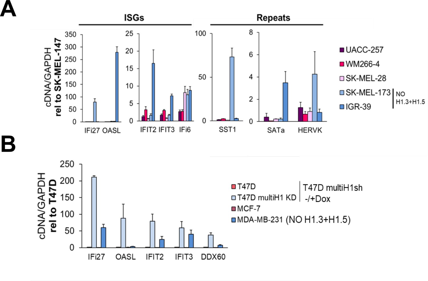
Cell lines lacking H1.3 and H1.5 show high basal expression of repetitive elements in comparison with cell lines with a complete H1 somatic repertoire.
(A) Reverse-transcriptase-quantitative PCR (RT-qPCR) of interferon stimulated genes (ISGs) and repetitive elements in different melanoma cell lines. Expression data are corrected by GAPDH and normalized by SK-MEL-147 cell line basal expression, which presents a complete H1 repertoire. SK-MEL-173 and IGR-39 cell lines show concomitant absence of H1.3 and H1.5 (see Figure 5—figure supplement 1C). (B) RT-qPCR of ISGs in breast cancer cell lines. MDA-MB-231 cell line does not express H1.3 and H1.5. Expression data are corrected by GAPDH and normalized by basal expression in T47D multiH1sh Untreated cells. T47D multiH1sh + Dox cells, which are reported to trigger a high expression of multiple ISGs (Izquierdo-Bouldstridge et al., 2017 in the main manuscript) are also shown for comparison.
Figure 6
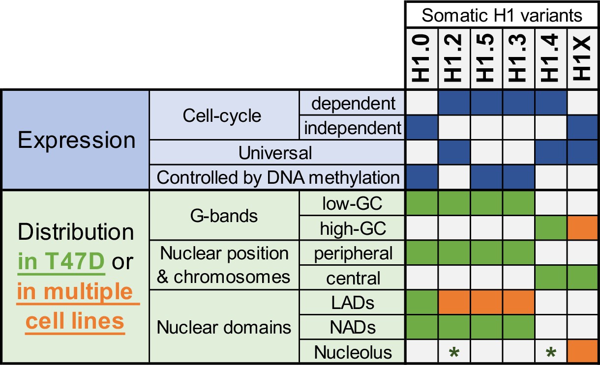
Summary of H1 variants expression and distribution specificities.
The table summarizes the main aspects of H1 variants expression (blue; top part) and distribution (green/orange; bottom part). Regarding distribution characteristics (from microscopy and ChIP-Seq experiments), green boxes indicate features observed in T47D breast cancer cells. If the association has been universally found in multiple human cell lines, it is highlighted in orange. Green asterisks indicate that, in T47D, phosphorylated H1.2 and H1.4 have been found to be enriched at nucleoli. Additional notes: Concomitant absence of H1.3 + H1.5 has been found in several cell lines, which also exhibit a redistribution of H1.4 and H1.0 to the nuclear periphery.
Additional files
-
Supplementary file 1
Oligonucleotides for semiquantitative PCR.
Forward (F) and reverse (R) oligonucleotides for the indicated genes are shown.
- https://cdn.elifesciences.org/articles/91306/elife-91306-supp1-v1.docx
-
MDAR checklist
- https://cdn.elifesciences.org/articles/91306/elife-91306-mdarchecklist1-v1.docx
Download links
A two-part list of links to download the article, or parts of the article, in various formats.
Downloads (link to download the article as PDF)
Open citations (links to open the citations from this article in various online reference manager services)
Cite this article (links to download the citations from this article in formats compatible with various reference manager tools)
Imaging analysis of six human histone H1 variants reveals universal enrichment of H1.2, H1.3, and H1.5 at the nuclear periphery and nucleolar H1X presence
eLife 12:RP91306.
https://doi.org/10.7554/eLife.91306.3


