Mapping the dynamics of force transduction at cell–cell junctions of epithelial clusters
- Harvard Medical School, United States
Figures
Figure 1
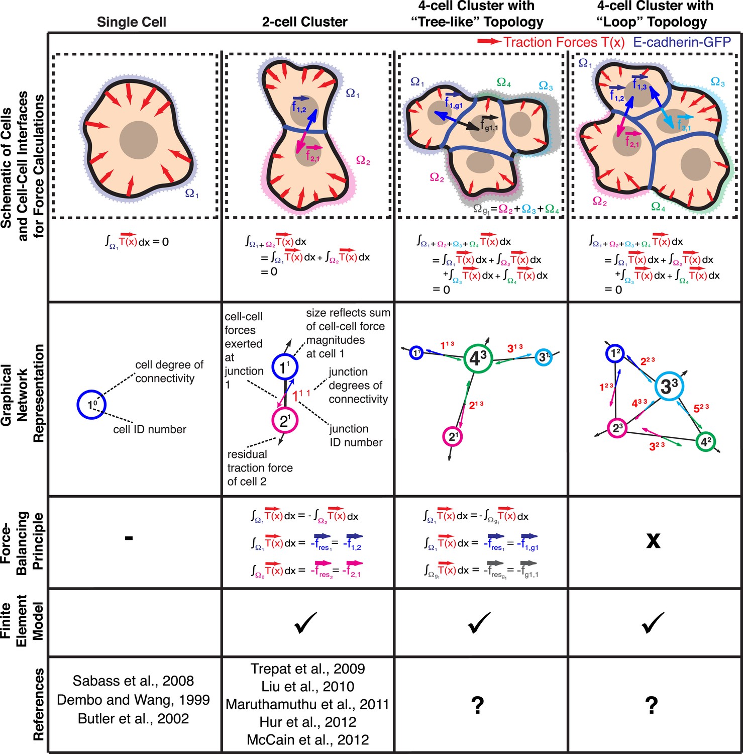
Calculation of cell–cell forces from traction forces.
Single cells and cell clusters (depicted in cartoon and graphical network representations for up to four cells, with areas Ω1–Ω4) exert traction forces on the substrate (red vectors; ). Integration of traction forces over the footprint (color-shaded boundaries) of a single cell (column 1) or an entire cell cluster (columns 2–4) yields a balanced net force of 0. In cell pairs and clusters with a ‘tree-like’ topology (columns 2 and 3), forces exchanged at each cell–cell junction can be determined by partitioning the cluster into two sub-networks and calculating the residual force required to balance the traction forces integrated over the footprint of each sub-network. See ‘Materials and methods’ for details. In cell clusters with a ‘loop’ topology (column 4), individual cell–cell junctions do not fully partition the cluster into disjoint sub-networks. In such cases, force transmission within a cell cluster can be calculated based on a model that describes the cluster as a thin-plate in mechanical equilibrium with the traction forces. The corresponding stress distribution inside the thin-plate is computed by the finite element method (FEM).
Figure 2
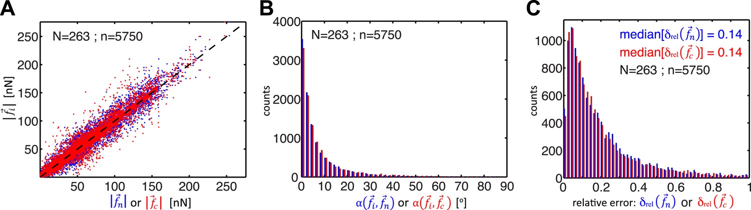
Comparison of cell–cell force calculations by force-balancing principle and by finite element modeling (FEM).
(A) Comparison of cell–cell force magnitudes as measured by the force balancing method (blue, is calculated from Equation 5) or FEM (red, ) vs the two independent measurements at each interface as predicted by force balancing calculations (= or ). Deviations of individual data from the dashed line indicate measurement errors. (B) Angular deviations between cell–cell forces as measured by the force balancing method (blue, ) or the FEM (red, ) and the two independent measurements at each interface as predicted by the force balancing calculations () (outliers (<3% of all data points) with angular deviations >90 degrees are not shown in the plot). (C) Relative error in cell–cell force measurements by the force balancing method (blue, ) or the FEM method (red, ). The median relative error for both measurement methods is 14% (outliers >100% relative error (<7% of all data points) are considered in the median calculation but are not shown in the plot). n = total number of measurements pooled from N distinct cell–cell junctions, with each junction having been measured over multiple time points.
Figure 3 with 1 supplement
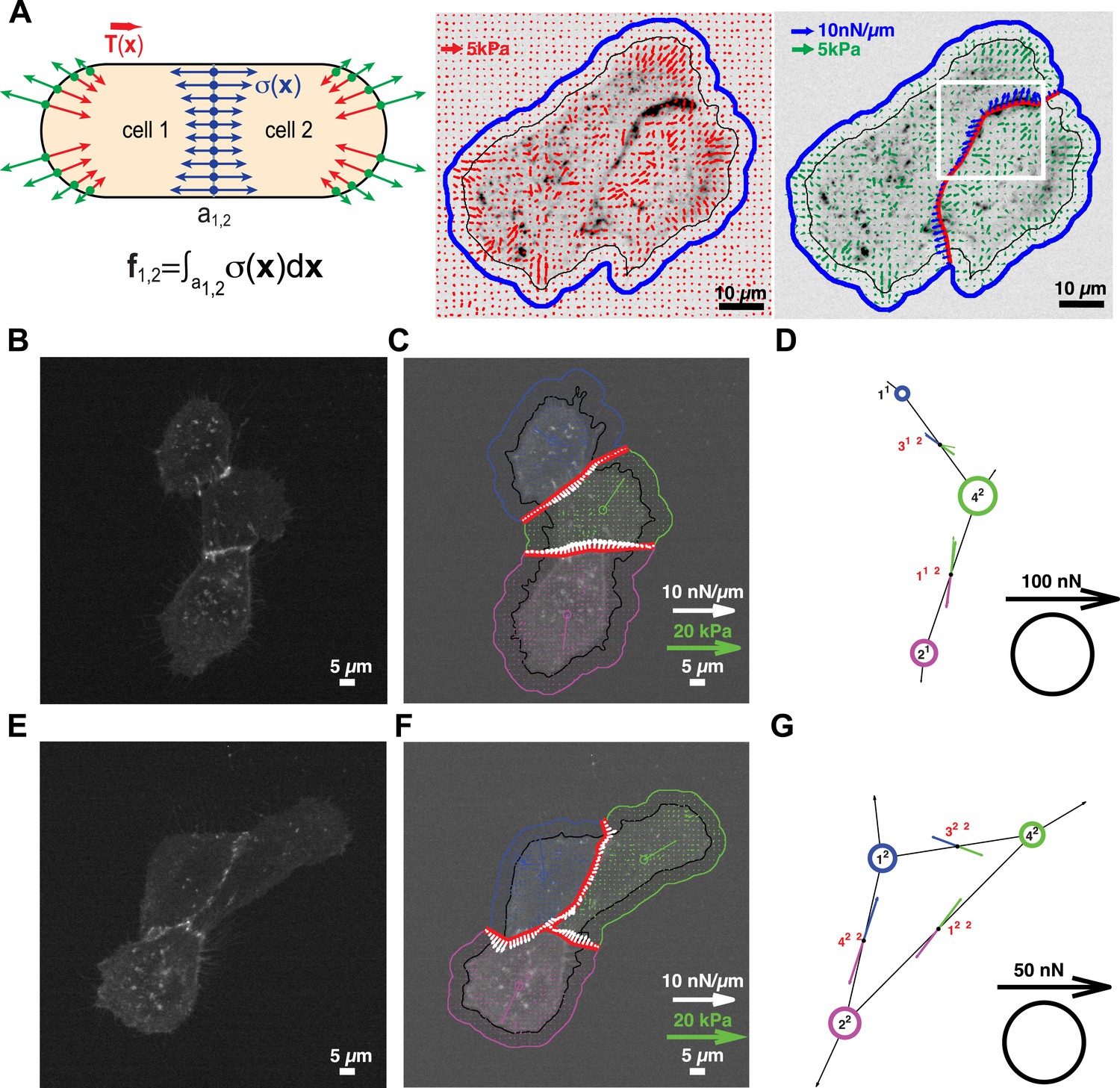
Quantification of cell–cell force exchange in a 3-cell cluster with changing topology.
(A) Schematic of the thin-plate model implemented to determine the stress profile along a cell–cell junction. Sign-inverted traction forces (green vectors) are applied to the thin-plate model to generate an internal stress distribution of cells 1 and 2 that is consistent with the measured traction forces (red vectors). The internal stress distribution is then used to calculate the force profile along the cell–cell interface a1,2 (blue vectors). See also Equation 13 in ‘Materials and methods’ section. Images show application of the approach to a cell pair. The cell–cell interface is marked by E-cadherin-GFP (inverted fluorescence signal). See also Video 1. White box: region of interest highlighted in Figure 6. Regularized FTTC was used for traction force reconstruction. (B) Image of an E-cadherin-GFP-expressing 3-cell cluster with ‘tree-like’ topology, which permits the calculation of force exchanges at each cell–cell junction by both the force-balancing principle and the thin-plate FEM modeling. (C) Segmentation of cells in the cluster, overlaid on the traction force field (small colored vectors) and an inverted fluorescence image of the cell cluster. Longer vectors in cell centers indicate residual traction forces for individual cells. Cell–cell stresses (white arrows) were calculated from sign-inverted traction forces. (D) Graphical network representation of the cluster. Dashed arrows at graph edge midpoints indicate the cell–cell force vector obtained from the force-balancing principle. Solid arrows of the same color show the corresponding cell–cell force vector derived from the thin-plate model. The difference between the two force estimates indicates the combined uncertainty of the two methods. See Figure 2 for error analysis over many clusters and junctions. (E–G) The same cluster as (B–D) at a different time point, when a junction formed between cell 1 and cell 2. This yields a loop topology preventing the calculation of cell–cell forces at junctions 1, 2, and 3 based on the force-balancing principle. See also Video 2.
Figure 3—figure supplement 1
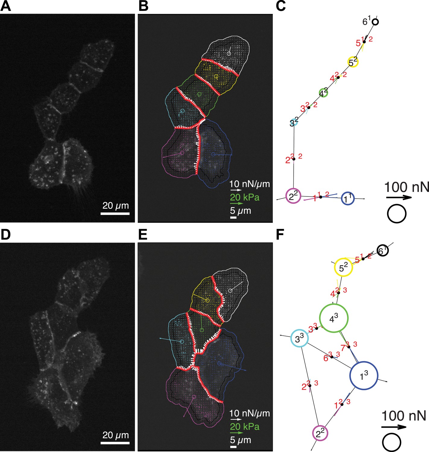
Quantification of cell–cell force exchange in a 6-cell cluster with changing topology.
(A) Image of an E-cadherin-GFP-expressing 6-cell cluster with ‘tree-like’ topology, which permits the calculation of force exchanges at each cell–cell junction by both the force-balancing principle and the thin-plate FEM modeling. (B) Segmentation of cells in the cluster, overlaid on the traction force field (small colored vectors) and an inverted fluorescence image of the cell cluster. Longer vectors in cell centers indicate residual traction forces for individual cells. Cell–cell stresses (white arrows) were calculated from inverted traction forces. (C) Graphical network representation of the cluster. Dashed arrows at graph edge midpoints indicate the cell–cell force vector obtained from the force-balancing principle. Solid arrows of the same color show the corresponding cell–cell force vector derived from the FEM. (D–F) The same cluster as (A–C) at a different time point, when two new junctions existed between cell 1 and cell 3, and cell 1 and cell 4, resulting in a loop topology. Cell–cell forces at junctions 1, 2, 3, 6, and 7 can no longer be derived based on the force-balancing principle. See also Video 3.
Figure 4 with 1 supplement
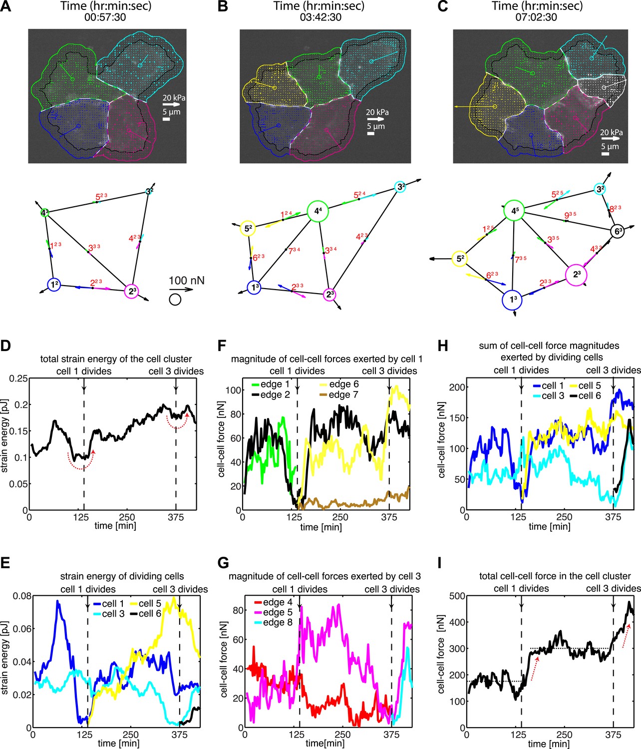
Force fluctuations in cell clusters during cell division.
(A–C) A 4-cell cluster undergoing two cell divisions (cell 1 divides into 1 and 5; cell 3 divides into 3 and 6). Top row, fluorescent images of E-cadherin-GFP signals overlaid with traction force field. Vectors originating from the center of each cell reflect the residual traction force of the cell. Bottom row, graphical network representations including residual traction force for each cell and junctional cell–cell forces (see Figure 1). (D–E) Total strain energy on the substrate exerted by the cell cluster and cells 1 and 3 before, during, and after the cell division events. (F–G) Cell–cell force magnitudes exerted by cells 1 and 3 on each of their cell–cell junctions. (H–I) Sum of cell–cell force magnitudes exerted by the whole cluster and cells 1 and 3 before, during, and after the cell division events. See also Figure 4—figure supplement 1 and Video 4.
Figure 4—figure supplement 1
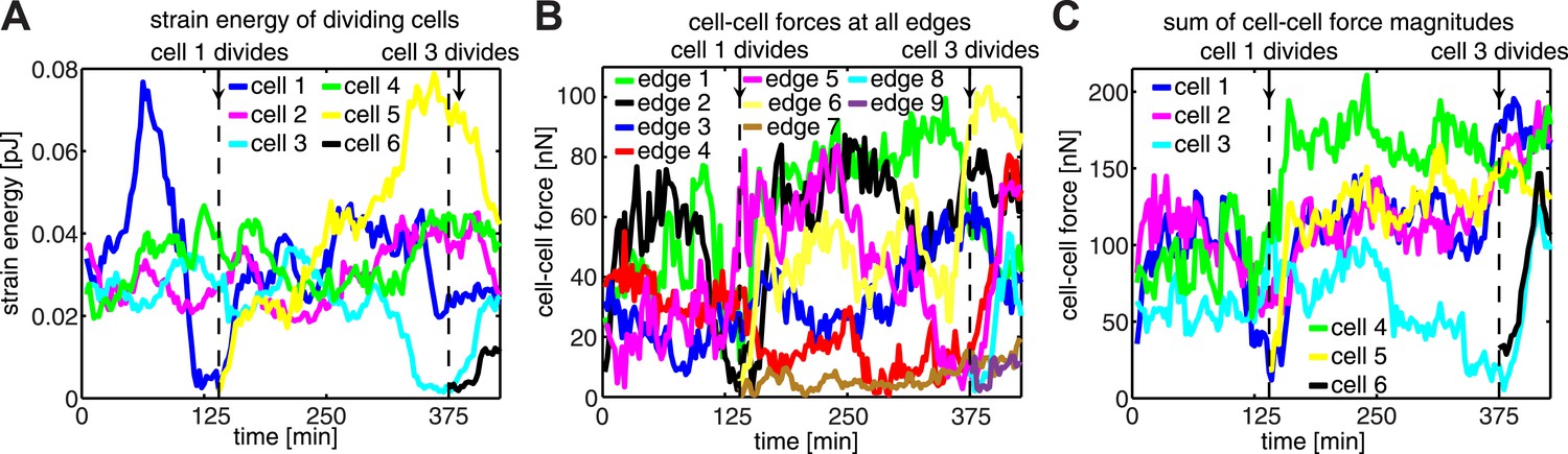
Force dynamics during cell divisions in cluster shown in Figure 4.
(A) Strain energies exerted by individual cells. (B) Fluctuations of cell–cell forces at individual junctions. (C) Total cell–cell forces exerted by individual cells.
Figure 5
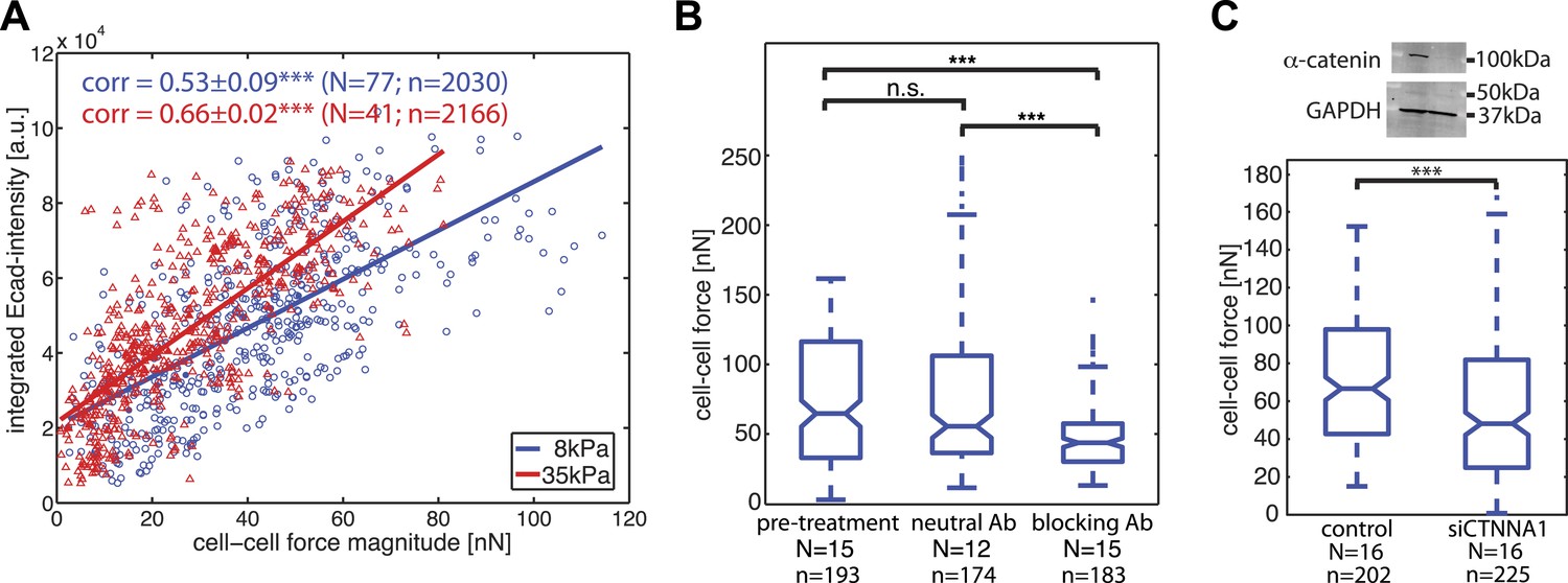
Correlation of calculated cell–cell forces with E-cadherin-GFP junctional localization.
(A) Correlation between E-cadherin-GFP intensity integrated along cell–cell interfaces and the corresponding interfacial force (integrated force profile), for cell clusters cultured on 8 kPa and 35 kPa substrates. Correlation coefficients were calculated from n measurements from N distinct cell–cell junctions pooled from multiple independent experiments. Plot displays only a subset of n measurements from one experiment. (B) Forces between cells treated with neutral and blocking antibodies against E-cadherin compared to forces before treatment. (C) Top: Western blot showing downregulation of alpha-catenin in cells transfected with siCTNNA1. Bottom: cell–cell forces between cells transfected with siCTNNA1 compared to those between control cells. N = number of cell–cell junctions measured; n = total number of measurements from N junctions. ***p < 0.005.
Figure 6 with 2 supplements
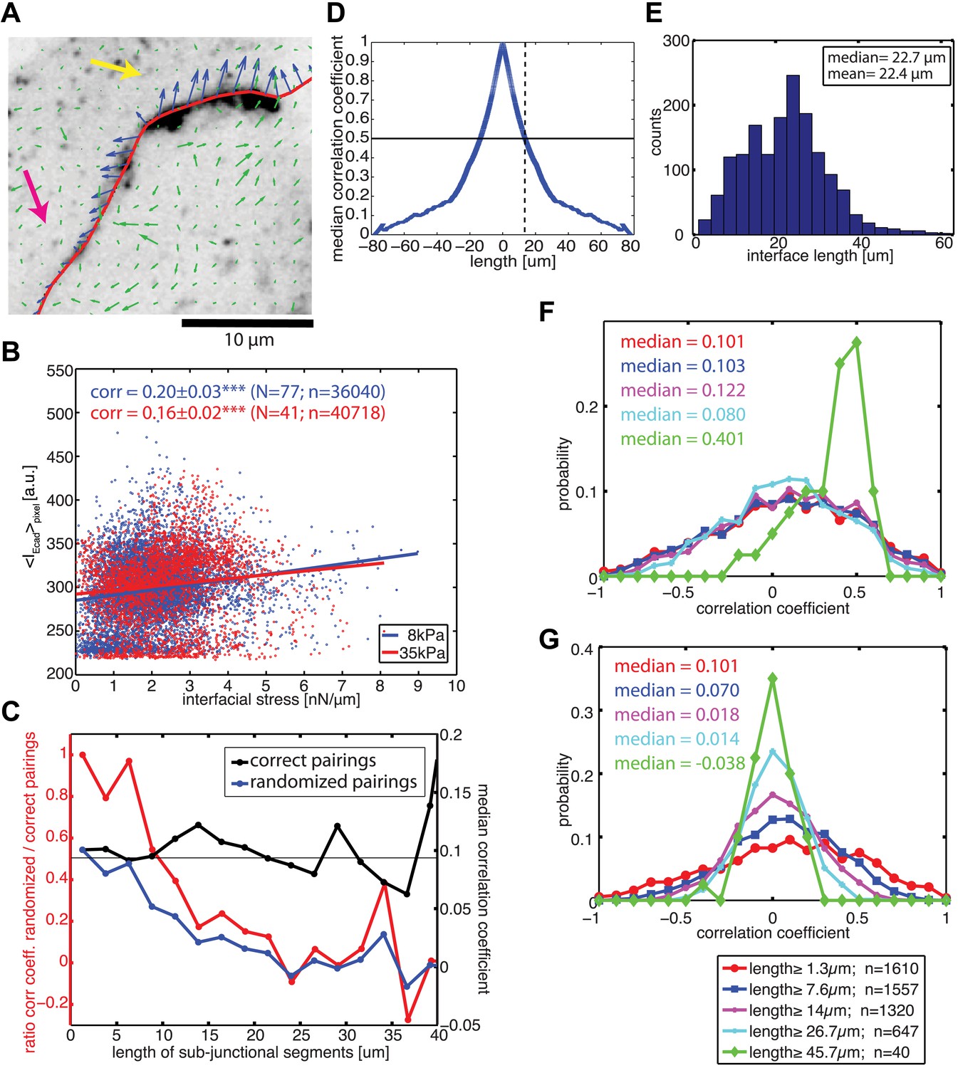
Correlation between calculated cell–cell forces at sub-junctional resolution and local E-cadherin-GFP intensities.
(A) E-cadherin-GFP intensity along a cell–cell junction overlaid by cell–cell stresses (blue) calculated by FEM (magnified region of interest indicated in Figure 3A). Green vectors: traction forces; yellow and magenta arrows highlight sub-junctional segments where high and low E-cadherin-GFP intensity correlated with high and low forces, respectively. (B) Correlation between local E-cadherin-GFP intensities and local calculated cell–cell forces for cell clusters cultured on 8 kPa and 35 kPa substrates. Correlation coefficients were calculated from n measurements from N distinct cell–cell junctions pooled from 5 independent experiments. For visualization purposes, the plot displays only a subset of the measurements extracted from one experiment. (C) Median correlation coefficients for correlation between local E-cadherin-GFP intensities and cell–cell forces calculated from sub-junctional segments of various lengths (correct pairings). Local E-cadherin-GFP intensities were then randomized within the sub-junctional segments of various lengths and correlated with calculated cell–cell forces from the corresponding segments (randomized pairings). The length-scale over which cell–cell stresses and E-cadherin intensity are coupled is estimated as the minimal sub-junctional segment length for which the ratio between the median correlation coefficient of randomized pairings and the median correlation coefficient of correct pairings drops below 0.5 (gray horizontal line), that is, randomization in shorter sub-junctional segments has no effect. Results were calculated from 77 junctions of 14 cell clusters cultured on 8 kPa substrates. (D) Autocorrelation of E-cadherin-GFP intensities along the same 77 junctions. Dotted line shows the sub-junctional length where the median autocorrelation coefficient drops below 0.5 (horizontal line). (E) Distribution of cell–cell junction lengths of 77 junctions, each measured over multiple time points. (F) Distribution of correlation coefficients between local E-cadherin-GFP intensities and cell–cell forces calculated from junctions of different lengths. (G) Distribution of correlation coefficients between local E-cadherin-GFP intensities and cell–cell forces randomized within junctions of different lengths. n = total number of measurements from 77 junctions of 14 cell clusters cultured on 8 kPa substrates. Similar results were found for cell clusters cultured on 35 kPa substrates (Figure 6—figure supplement 1).
Figure 6—figure supplement 1

Correlation between calculated cell–cell stresses and local E-cadherin-GFP intensities along junctions of cell clusters cultured on 35 kPa substrates.
(A) Median coefficient of correlation between local E-cadherin-GFP intensities and cell–cell stresses calculated from sub-junctional segments of various lengths (correct pairings). Calculated cell–cell stresses were then randomized within the sub-junctional segments of various lengths and correlated with local E-cadherin-GFP intensities from the corresponding segments (randomized pairings). The length-scale over which cell–cell stresses and E-cadherin intensity are coupled is estimated as the minimal sub-junctional segment length for which the ratio between the median correlation coefficient of randomized pairings and the median correlation coefficient of correct pairings drops below 0.5 (gray horizontal line), that is, randomization in shorter sub-junctional segments has no effect. This length-scale may also be considered an upper limit of resolution for the cell–cell stress calculation by FEM. (B) Autocorrelation of E-cadherin-GFP intensities along cell–cell junctions. Dotted line shows the sub-junctional length where the median autocorrelation coefficient drops below 0.5 (horizontal line). (C) Distribution of cell–cell junction lengths. (D) Distribution of correlation coefficients between local E-cadherin-GFP intensities and cell–cell stresses calculated from junctions of different lengths. (E) Distribution of correlation coefficients between local E-cadherin-GFP intensities and cell–cell stresses randomized within junctions of different lengths. n = total number of measurements from 41 junctions of 10 cell clusters.
Figure 6—figure supplement 2

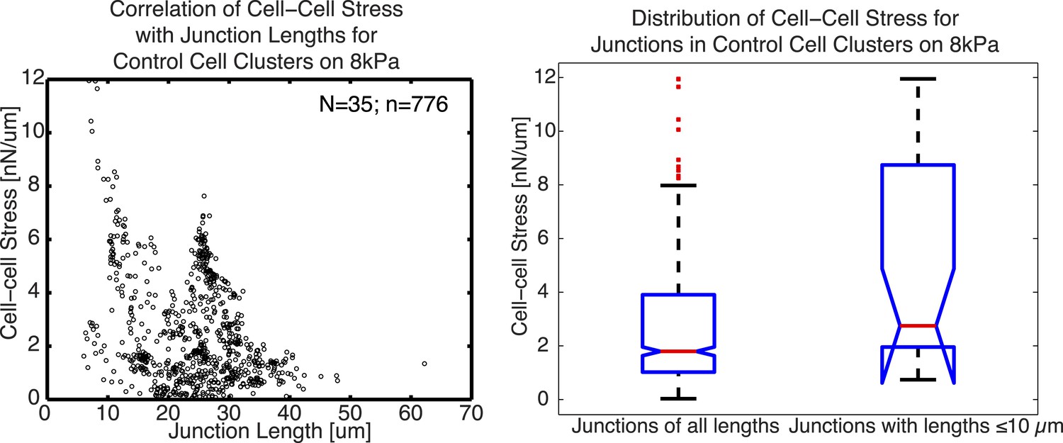
Relationship between cell–cell stress and junction length.
(A) Cell–cell stresses as a function of junction lengths for control cell clusters on 8 kPa substrates. (B) Distribution of cell–cell stresses for junctions of all lengths and junctions with lengths less than or equal to 10 µm. n = total number of measurements from N distinct junctions. Only junctions with a minimal degree of connectivity =1 were used in both plots to avoid potential false attribution of cell–cell stress from adjoining junctions.
Figure 7
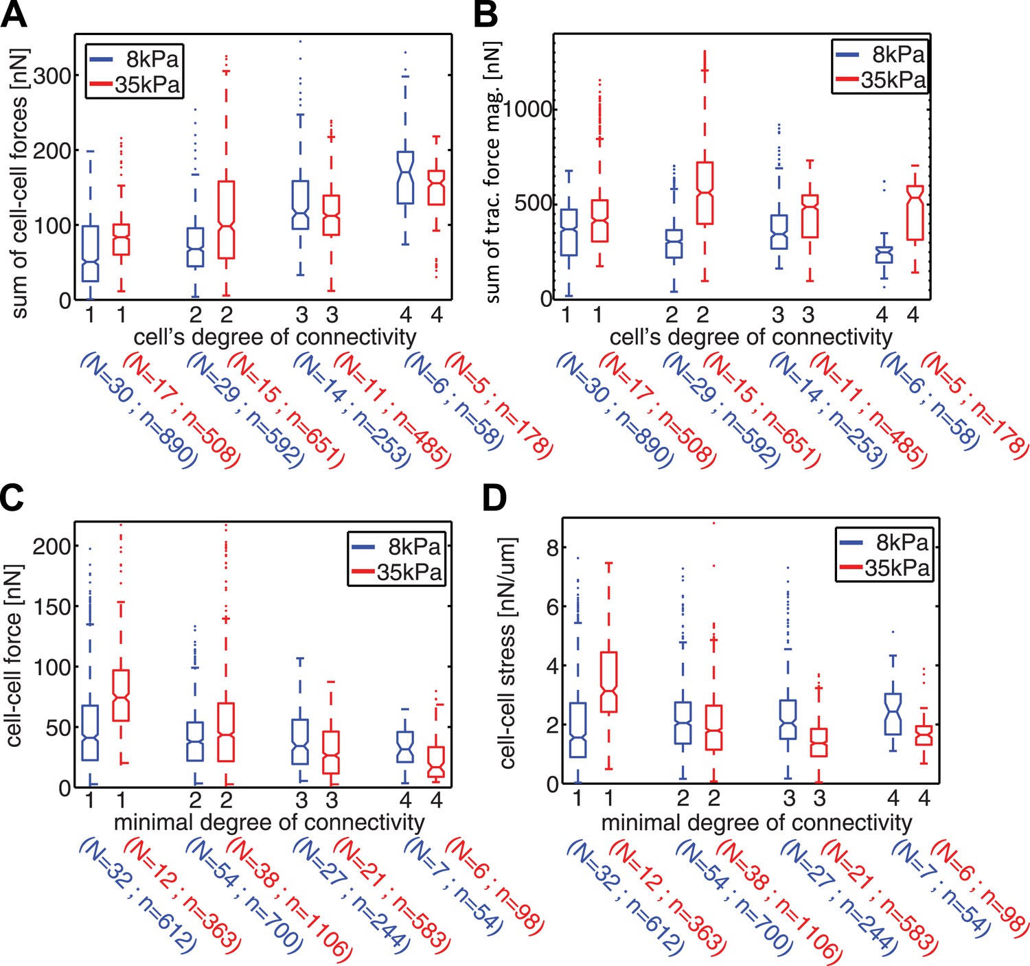
Spatial organization of cell–cell forces in clusters.
(A–B) The sum of cell–cell force magnitudes (A) and traction force magnitudes (B) for cells connected to 1, 2, 3, or 4 neighbors (degree of connectivity k). (C) Force magnitudes at individual cell–cell junctions, classified according to the minimal degree of connectivity (smaller of the k values for the two connected cells). (D) Stress at individual cell–cell junctions, classified according to the minimal degree of connectivity. Center line within box represents median, notches indicate the 95% confidence interval about median. Non-overlapping notches between samples indicate that the sample medians differ with statistical significance at the 5% level. Lower and upper bounds of box indicate first and third quartiles. Whiskers indicate 1.5 times inter-quartile range. Points outside the whiskers represent outliers. n = total number of measurements from N distinct cells or junctions.
Figure 8

Localization of focal adhesions and cell–cell adhesions in MCF10A cell clusters.
(A–B) Focal adhesions in a representative MCF10A cell pair (A) and 4-cell cluster visualized by immunostaining of paxillin, cell–cell junctions visualized by E-cadherin-GFP. Fluorescence images were acquired using the same parameters as for TFM measurements.
Figure 9 with 1 supplement
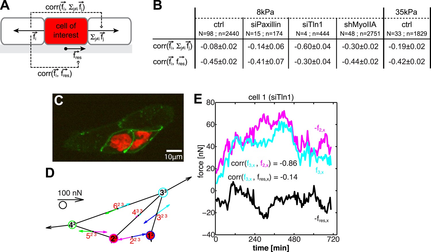
Dynamic force transmission through cells.
(A) Schematic of temporal cross-correlation analysis of force fluctuations at opposing cell–cell junctions. To determine the extent of force transmission from one cell–cell junction across a cell (depicted here in red) to the next junction or to the cell substrate, force fluctuations at one cell–cell interface i of the cell-of-interest are correlated with the fluctuations of the vector sum of cell–cell forces at all remaining cell–cell junctions of this cell or with the fluctuations of the negative residual traction force of the cell, respectively. See ‘Materials and methods’ for details. (B) Cross-correlation analysis results for control cells on 8 kPa or 35 kPa substrates and for cells with downregulation of paxillin (siPax), talin-1 (siTln1), or myosin-IIA (shMyoIIA) in mosaic cell clusters on 8 kPa substrates. See Figure 9—figure supplement 1. (C) Mosaic cell cluster with two siTln1-treated cells (red nuclei). (D) Graphical network representation of the cluster at the same time point. See Video 5 for full time lapse sequence. (E) Time courses of x-component of junctional forces (junction 2, magenta; junction 3, cyan) and residual traction force (black) in target cell 1 (cf. graphical network in D).
Figure 9—figure supplement 1
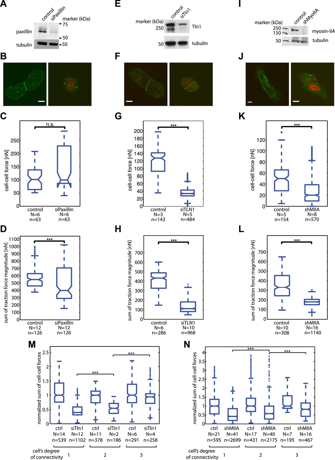
Mosaic downregulation of paxillin, talin-1, and myosin-IIA.
(A) Western blot showing downregulation of paxillin in cells transfected with siPax. (B) E-cadherin-GFP-expressing cell pairs without (left) or with paxillin downregulation (marked by red nuclei). (C) Cell–cell force magnitudes at junctions between control or siPax cells. (D) Sum of traction force magnitudes exerted by individual control or paxillin-downregulated cells in cell pairs. (E) Western blot showing downregulation of talin-1 in cells transfected with siTln1. (F) E-cadherin-GFP-expressing cell pairs without (left) or with talin-1 downregulation (marked by red nuclei). (G) Cell–cell force magnitudes at junctions between control or siTln1 cells. (H) Sum of traction force magnitudes exerted by individual control or talin-1-downregulated cells in cell pairs. (I) Western blot showing knock-down of myosin-IIA in cells transfected with shRNA targeting the protein. (J) E-cadherin-GFP-expressing cell pairs without (left) or with myosin-IIA downregulation (marked by red nuclei). (K) Cell-cell force magnitudes at junctions between control or myosin-IIA-downregulated cells. (L) Sum of traction force magnitudes exerted by individual control or myosin-IIA-downregulated cells in cell pairs. (M) Sum of cell–cell force magnitudes at individual control or talin-1-downregulated cells with various degrees of connectivity. (N) Sum of cell–cell force magnitudes at individual control or myosin-IIA-downregulated cells with various degrees of connectivity. N = number of distinct junctions or cells measured; n = total number of measurements from N junctions or cells. ***p << 0.05.
Author response image 1
Author response image 2
Videos
Video 1
Force exchange between E-cadherin-GFP-expressing MCF10A cell pair quantified at sub-junctional resolution using FEM; related to Figure 3A.
Measured traction stresses (green vectors) were inverted for the calculation of mechanical stress distribution within the cell pair based on the thin-plate model, and the calculated cell internal stresses were integrated along the cell–cell junction to obtain the transmitted cell–cell stress profile along the junction (blue vectors; see ‘Materials and methods’ for details). Both the traction stress map and the stress profile were overlaid onto transmitted light (left) and E-cadherin-GFP fluorescence (right) images. The cell–cell junction is outlined by the red line, while the boundary of the cell pair is outlined by the black line (tight cluster mask). The blue outline represents the dilated cluster mask employed to capture the entire traction force field generated by the cell pair. Images were acquired one frame every 8 min for over 2 hr and 40 min with a 40× 0.95 NA air objective using a spinning disk confocal microscope; frame display rate =3 fps.
Video 2
Force exchanges in a three-cell MCF10A cluster with changing topology; related to Figure 3.
(Left) E-cadherin-GFP fluorescence. (Middle) Cell–cell stresses (white vectors) and traction forces (colored vectors) overlaid on fluorescence images. The cell–cell junctions are outlined in red. Vectors originating from cell centers reflect the residual traction forces of each cell. See ‘Materials and methods’ for details. (Right) Network representation of the cluster indicating the residual traction force of each cell and the reconstructed cell–cell forces along junctions. Solid thick color vectors represent integrated cell–cell forces calculated using the FEM approach; dotted thin color vectors represent cell–cell forces calculated using the force-balancing principle. Note the force-balancing principle is insufficient for calculating junctions that are in a ‘loop’ configuration. Vector lengths and circle sizes represent force magnitudes. Images were acquired one frame every 4 min for 2 hr with a 40× 0.95 NA air objective using a spinning disk confocal microscope; frame display rate =3 fps.
Video 3
Force exchanges in a six-cell MCF10A cluster with changing topology; related to Figure 3—figure supplement 1.
(Left) E-cadherin-GFP fluorescence. (Middle) Cell–cell stresses (white vectors) and traction forces (colored vectors) overlaid on fluorescence images. The cell–cell junctions are outlined in red. Vectors originating from cell centers reflect the residual traction forces of each cell. See ‘Materials and methods’ for details. (Right) Network representation of the cluster indicating the residual traction force of each cell and the reconstructed cell–cell forces along junctions. Solid thick color vectors represent integrated cell–cell forces calculated using the FEM approach; dotted thin color vectors represent cell–cell forces calculated using the force-balancing principle. Note the force-balancing principle is insufficient for calculating junctions that are in a ‘loop’ configuration. Vector lengths and circle sizes represent force magnitudes. Images were acquired one frame every 7 min for >3 hr with a 40× 0.95 NA air objective using a spinning disk confocal microscope; frame display rate =3 fps.
Video 4
Force exchange in a four-cell MCF10A cluster with two cell divisions; related to Figure 4.
(Left) E-cadherin-GFP fluorescence. (Middle) E-cadherin-GFP fluorescence images overlaid with traction forces (small colored vectors). Tight cluster mask (black) and dilated (colors) cell outlines are also overlaid. Vectors originating from cell centers reflect the residual traction forces of each cell. (Right) Network representation of the cluster indicating the residual traction force of each cell and the reconstructed cell–cell forces along junctions. Vector lengths and circle sizes represent force magnitudes. Images were acquired one frame every 2.5 min over a time course of 7 hr with a 40× 0.95 NA air objective using a spinning disk confocal microscope; frame display rate =18 fps.
Video 5
Force exchange in four-cell cluster with mosaic downregulation of talin-1 on 8 kPa substrates; related to Figure 9C–E.
(Left) E-cadherin-GFP fluorescence (green). Cells with talin-1 knock-down are also labeled with H2B-mCherry (red). (Middle) E-cadherin-GFP fluorescence images overlaid with traction forces (small colored vectors). Tight cluster mask (black) and dilated (colors) cell outlines are also overlaid. Vectors originating from cell centers reflect the residual traction forces of each cell. (Right) Network representation of the cluster indicating the residual traction force of each cell and the reconstructed cell–cell forces along junctions. Vector lengths and circle sizes represent force magnitudes. Images were acquired one frame every 4.5 min over a time course of >10 hr with a 40× 0.95 NA air objective using a spinning disk confocal microscope; frame display rate =18 fps.
Additional files
-
Source code 1
MATLAB analysis codes.
- https://doi.org/10.7554/eLife.03282.024
Download links
A two-part list of links to download the article, or parts of the article, in various formats.
Downloads (link to download the article as PDF)
Open citations (links to open the citations from this article in various online reference manager services)
Cite this article (links to download the citations from this article in formats compatible with various reference manager tools)
Mapping the dynamics of force transduction at cell–cell junctions of epithelial clusters
eLife 3:e03282.
https://doi.org/10.7554/eLife.03282


