Habitat and social factors shape individual decisions and emergent group structure during baboon collective movement
- Princeton University, United States
- Max Planck Institute for Ornithology, Germany
- University of Konstanz, Germany
- University of Oxford, United Kingdom
- University of California, Davis, United States
- Smithsonian Tropical Research Institute, Panama
Figures
Figure 1

Combining three-dimensional habitat reconstruction with baboon tracking data to determine which habit and social features predict individual movement decisions.
(A) Example of baboon trajectories overlaid on a high-resolution three-dimensional habitat reconstruction. Colored lines show trajectories of each baboon. (B) Predictive accuracy for step selection models using habitat features only (red point), social features only (blue point), or both social and habitat features (purple point), as compared to a null model (black point). Y-axis shows the negative log loss of out-of-sample data; points farther up the y-axis indicate better model predictions. (C) AIC weights associated with each feature based on multi-model inference. Each point shows the feature weights for a particular baboon individual, and black bars show the median feature weight across all individuals. Features are ranked from highest median feature weight (top) to lowest mean feature weight (bottom). See also Videos 1–2.
Figure 2
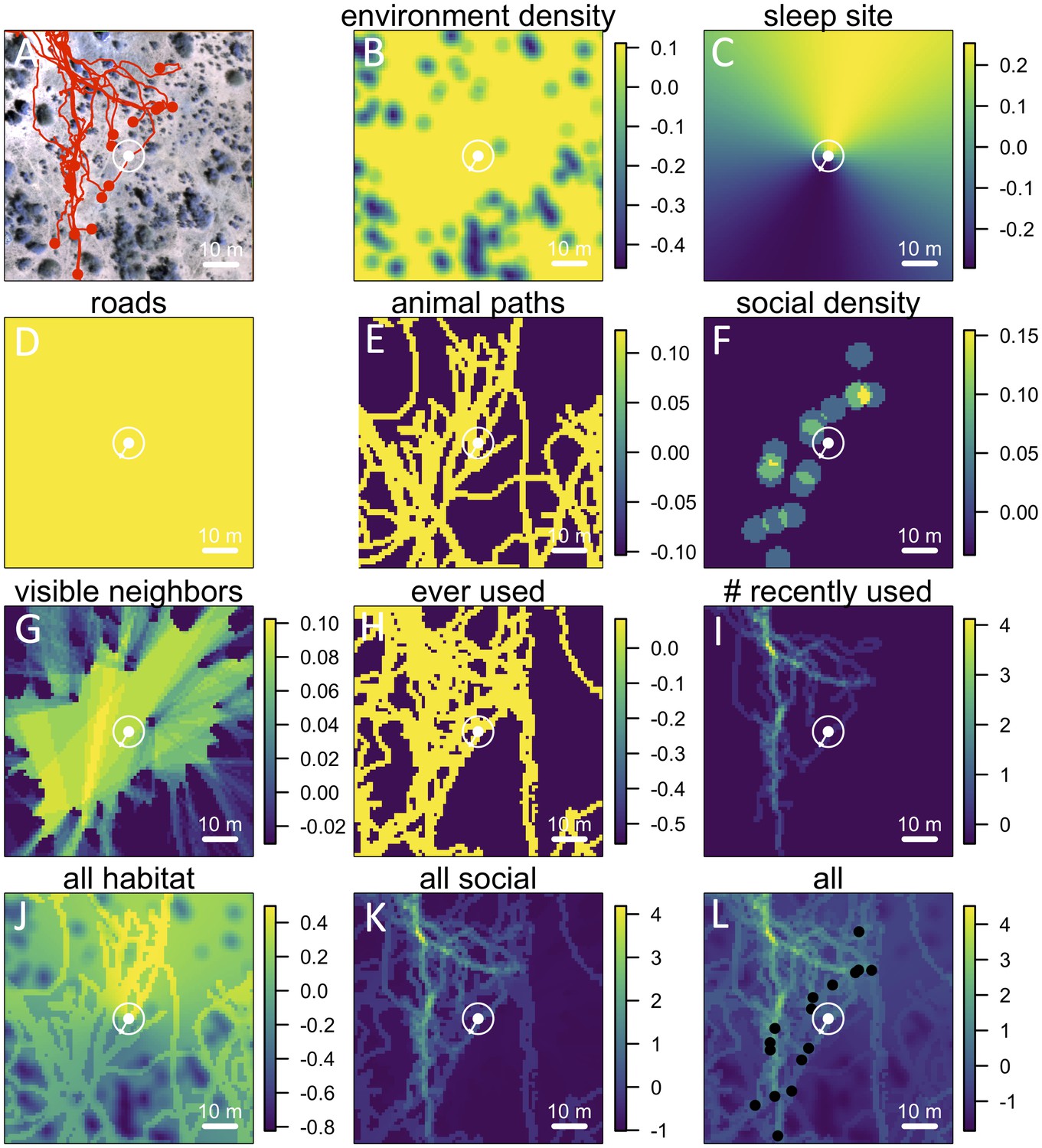
Visualizing the preference landscape underlying individual movement decisions.
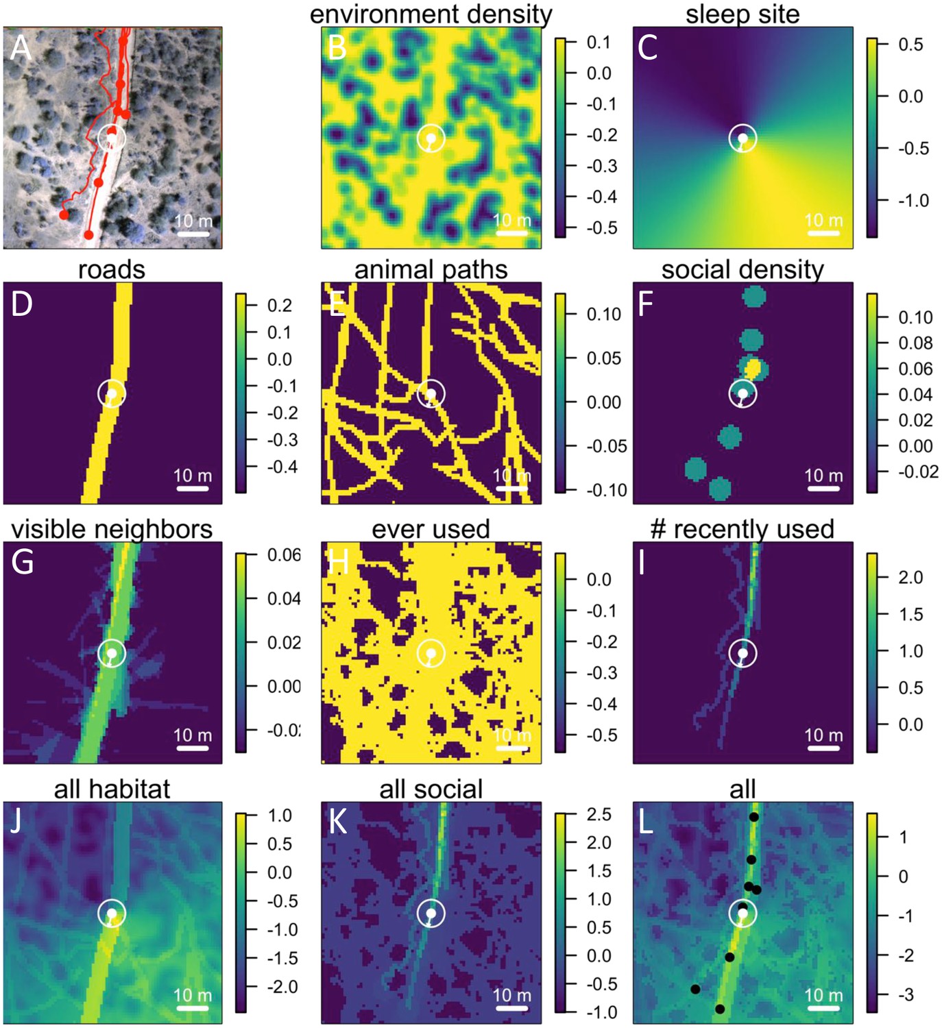
(A) Example of a single step taken by a focal individual. Background image shows overhead view of 3D habitat reconstruction. White marker shows the location of the focal baboon (whose next step is being modeled), and white circle shows a radius of 5 m (the specified step size) around the focal individual. White arrow shows the step actually taken by the individual. Red lines show recent locations of other baboons, and red points show locations of other baboons at the end of the step. (B –I) Visualizations of the influence of each habitat and social factor (the ‘preference landscape’) based on the fitted step selection model - lighter yellow areas represent locations that are more preferred, and darker blue areas are less preferred. Each panel represents the influence of a particular factor (ignoring all others) as predicted by the model: (B) vegetation density, (C) sleep site direction, (D) roads, (E) animal paths, (F) social density, (G) fraction of visible neighbors, (H) locations that have ever been used by another baboon, (I) number of baboons that have recently (in the past 4.5 minutes) used a location. (J–L) Last three panels represent overall preference landscapes, combining information from all habitat features only (J), all social features only (K), and all features, i.e. the full model prediction (L). For another example of preference landscapes (from a case where the focal individual started on a road), see Appendix 1—figure 14.
Figure 3

The interplay between habitat and social features in shaping individual movement decisions.
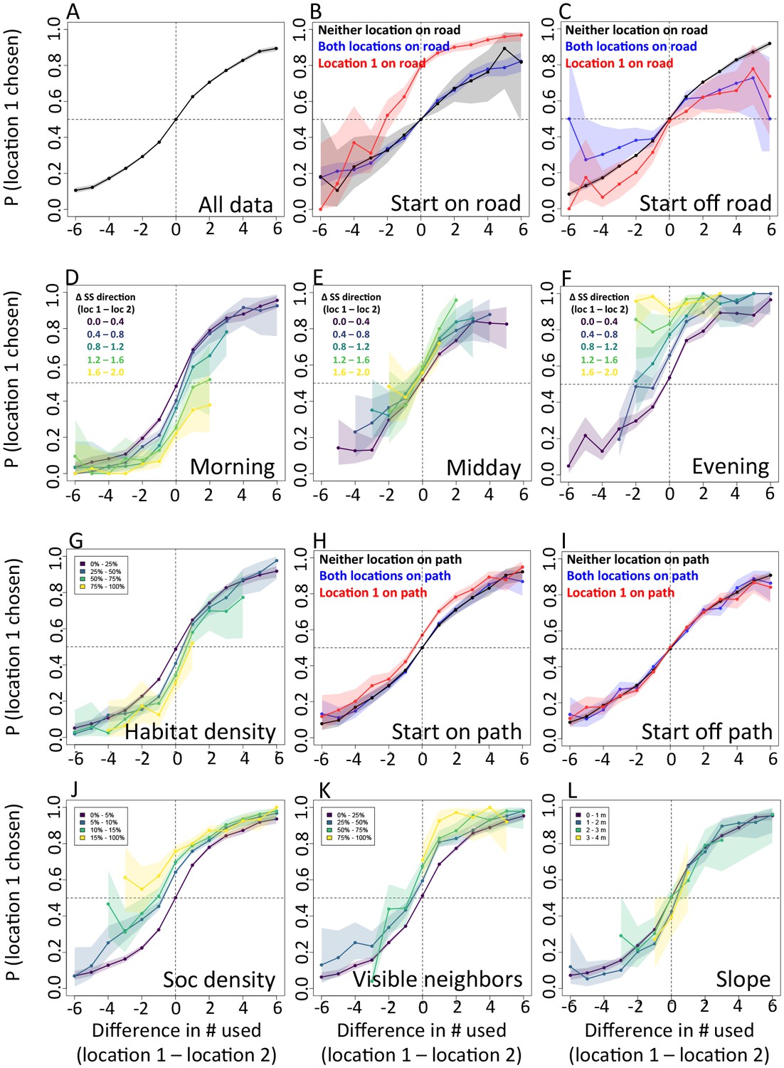
We compare each real location where a baboon moved to an alternative location that it could have moved. We randomly select one of these two locations and denote it location 1, denoting the other location 2. Each plot shows the probability that location 1 was the true location actually chosen by the baboon, as a function of the difference between the numbers of other baboons that had recently (within the past 4.5 min) occupied location 1 and the number that had recently occupied location 2. (A) Across all data, the location chosen by the focal baboon is more likely to be the one recently occupied by more of its group mates. Moreover, the greater the difference between the number of baboons to have occupied each location, the stronger the effect (sigmoidal shape of curve). (B,C) Movement decisions are altered by the influence of roads. Here, data are shown from when the focal baboon started on a road (B) and when it started off a road (C), in three different cases: neither location was on a road (black line), both locations were on a road (blue line) or location 1 was on a road whereas location 2 was not (red line). (D–F) Movement decisions are influenced by the direction of the sleep site in the morning (D) and evening (F), but less in the midday (E). Each colored line shows data from instances when the difference in the steps’ directedness toward the sleep site between location 1 and location 2 fell into a different bin (given in the legend), with lighter (more yellow) colors indicating a greater difference. When there is little difference (dark purple lines), the curve resembles that shown in panel A. As the difference increases, the location that is in the direction away from (in the morning) or towards (in the evening) the sleep site becomes more likely to be chosen by the baboon. Shaded regions denote 95% confidence intervals (based on Clopper-Pearson intervals). See also Appendix 1—figure 12 (other environmental influences) and Appendix 1—figure 13 (10 m steps rather than 5 m steps).
Figure 4
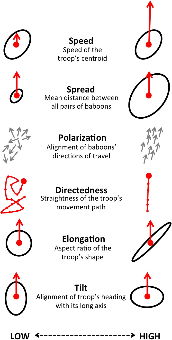
Illustration of the six measures used to characterize group-level properties.
For further information, see Supplementary methods.
Figure 5

At the group level, troop structure and movement changes based on roads and vegetation density.
(A) Two-dimensional histograms of the speed and polarization (top panel), spread and directedness (middle panel), and elongation and tilt (bottom panel) of the baboon troop across all data. Lighter areas represent more likely group configurations. (B–C) Difference between the distributions within a given context and the overall distribution across all data. Redder areas represent group configurations that are over-represented within a given context (relative to the rest of the data), and bluer areas represent under-represented configurations. Each column represents a different context: (B) on-road and off-road, and (C) open, medium, and dense vegetation. See also Appendix 1—figures 17–18 for the influence of path density and time of day respectively, as well as Appendix 1—figures 19–22 for one-dimensional histograms of each group-level property within each context.
Figure 6
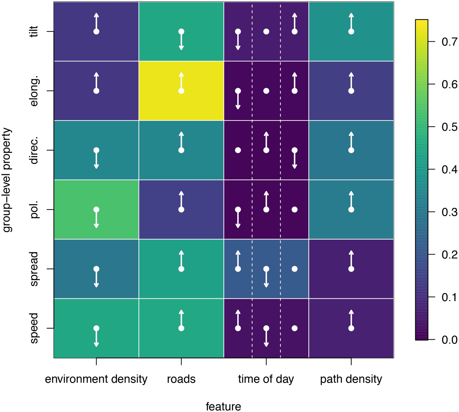
Results of fitting linear models to predict group-level properties as a function of features of the habitat occupied by the group and the time of day.
Colors show feature weights, with lighter colors indicating habitat/temporal features (columns) that were more supported by multi-model inference to predict each group-level property (rows). Arrows indicate the direction of the effects for each fit, with upward (downward) pointing arrows indicating a positive (negative) effect. For time of day column, arrows correspond to morning (left), midday (middle), and evening (right), with the upward (downward) pointing arrow indicating the time of day associated with the largest (smallest) value of the group-level property in each row.
Appendix 1—figure 1

Drone-mapped area and identification of roads and sleep site locations.
(A) UAV-mapped area in relation to troop range during the entire period of tracking. Each thin colored line represents the daily trajectory of a single baboon, and different colors represent different days (though 35 days of tracking data are shown here, only the first 14 days of data were used in the analysis). Thick white lines enclose the UAV-mapped region, for which we generated a three-dimensional habitat reconstruction (see Figure 1A). (B) Map showing the locations of roads (red lines), the river (blue line), and the troop’s sleep site (yellow circles indicate the troop’s sleeping location on each morning, defined as the centroid of all baboon locations).
Appendix 1—figure 2

Processing 3-dimensional habitat reconstruction.
Starting with the 3-dimensional habitat reconstruction data (A), we used a ground the classification algorithm MCC-LIDAR to identify non-ground points (B). We then rasterized these data to a grid with 20 × 20 cm pixels (C). Here, black pixels indicate ground and white pixels indicate non-ground. Using image segmentation, we identified connected clusters of pixels (D), here represented as sections of different colors (with the ground here represented in blue). We then removed all identified objects smaller than 2 m2 to reduce small-scale noise (E). (F) shows the baboon trajectories (in red) overlaid on the processed image.
Appendix 1—figure 3
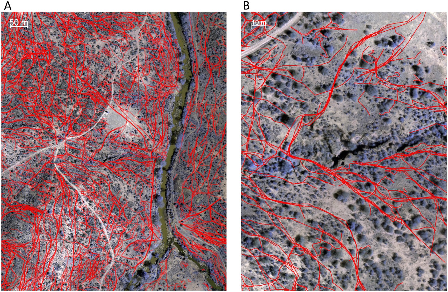
Identifying animal paths.
Animal paths, shown in red here, were traced out manually from the orthomosaic images using Google Earth Pro. (A) and (B) show a large area and zoomed in region, respectively.
Appendix 1—figure 4
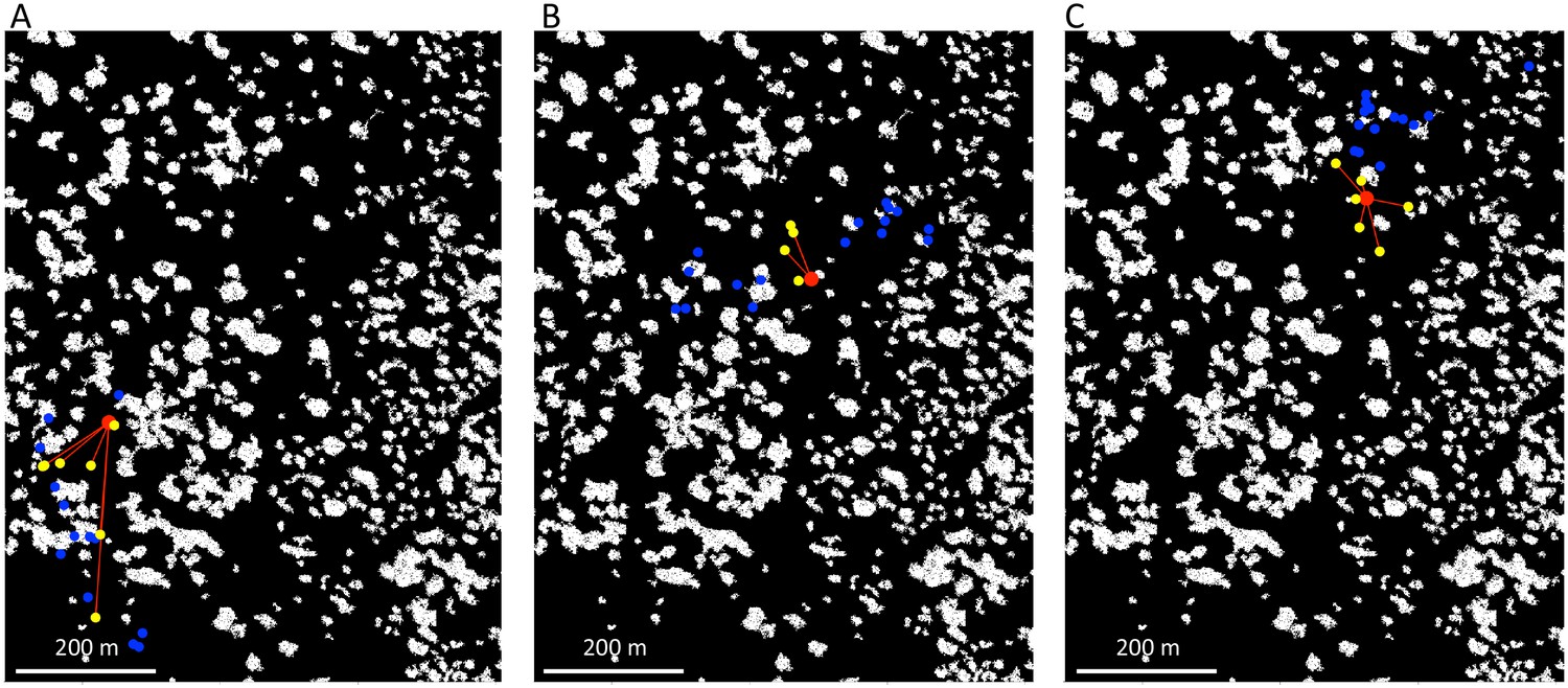
Estimating which baboons are visible from a given location.
We estimated the direct line-of-sight from a given focal location (red marker), assuming that if this line-of-sight crossed through any non-ground pixels, it was blocked. Here, yellow markers show baboons that are visible from the focal location, with red lines connecting them. Blue markers show baboons that are out-of-sight from the focal location. Each panel corresponds to a different time, as the baboons move across the landscape.
Appendix 1—figure 5
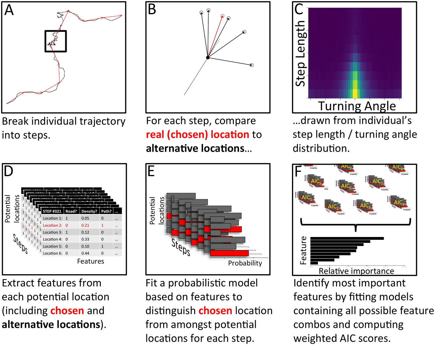
Analysis pipeline for determining which features are most important in predicting individual baboons’ decisions, using a step selection analysis and multi-model inference.
To model a given baboon, its trajectory is first broken up into a series of steps using spatial discretization (A). Black line shows the full trajectory, and red lines show the spatially discretized steps. Square encloses one step. (B) For each step, the real location chosen by the baboon (red) is then compared to a set of alternative options (black), with these options drawn from that individual’s empirical step length / turning angle distribution (C). Features (such as whether the location is on a road, the vegetation density, how many baboons are within a certain range, etc.) are then extracted from each potential location, across all steps (D). A conditional logistic regression model predicting the probability that the baboon chose each alternative option based on the features of all options (E) is then fit using maximum likelihood. (F) Models containing all possible combinations of features are fit in this way, and their AIC scores computed. The relative importance of each feature in the models is then determined by computing the AIC weight of each feature across all models. Features that are present in many of the best models receive the largest weights.
Appendix 1—figure 6
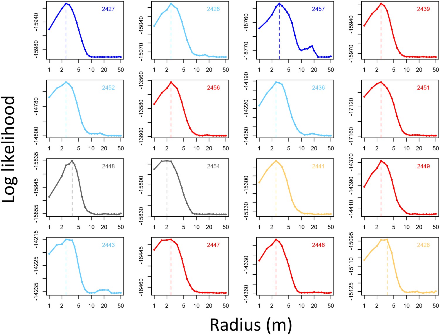
Determining the spatial scale over which environment density predicts baboon movement decisions.
For each baboon (individual panels), models predicting baboon movement decisions from the environment density (density of non-ground pixels within a radius R) were fit across a range of possible radii. Plots show the log maximum likelihood of models (y-axis) for each value of R (x-axis), with the peak value representing the environment density scale best supported by the data.
Appendix 1—figure 7
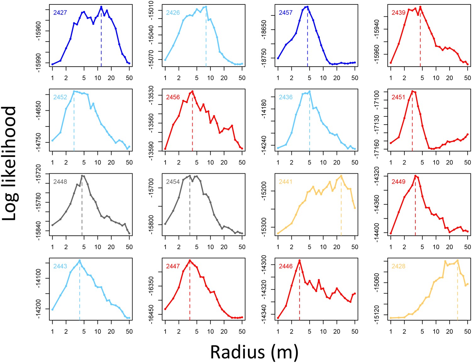
Determining the spatial scale over which social density (the fraction of other baboons within a given radius of a potential location) predicts baboon movement decisions.
For each baboon (individual panels), models predicting baboon movement decisions from the social density (fraction of other baboons within a radius R) were fit across a range of possible radii. Plots show the log maximum likelihood of models (y-axis) for each value of R (x-axis), with the peak value representing the social density scale best supported by the data.
Appendix 1—figure 8
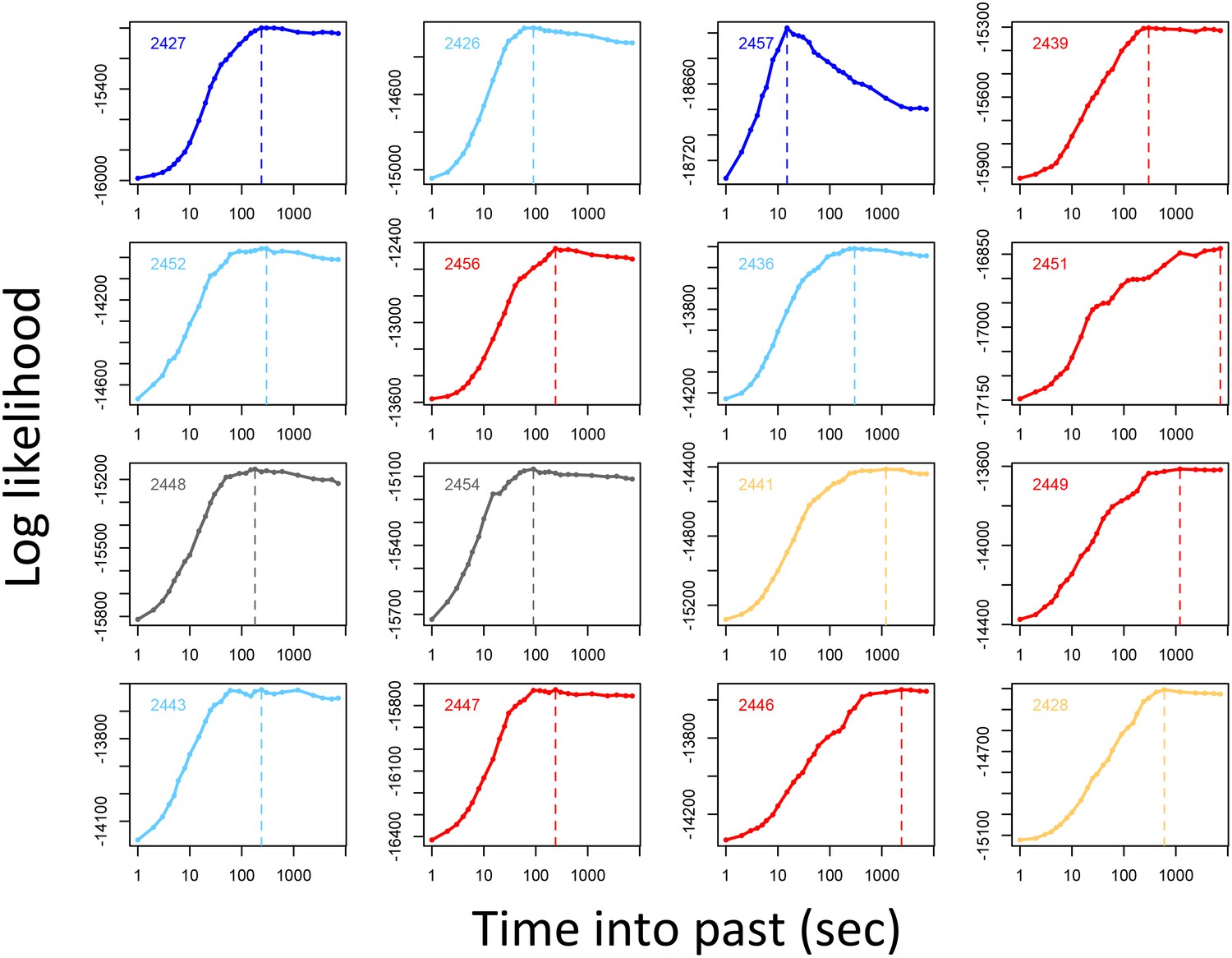
Determining the temporal scale over which the previous locations of other baboons predicts baboon movement decisions.
For each baboon (individual panels), models of baboon movement decisions were fit using the number of baboons to occupy a potential location within a certain window of time into the past as a predictor variable, across a range of time windows. Plots show the log maximum likelihood of models (y-axis) for each time window (x-axis), with the peak value representing the temporal scale best supported by the data.
Appendix 1—figure 9
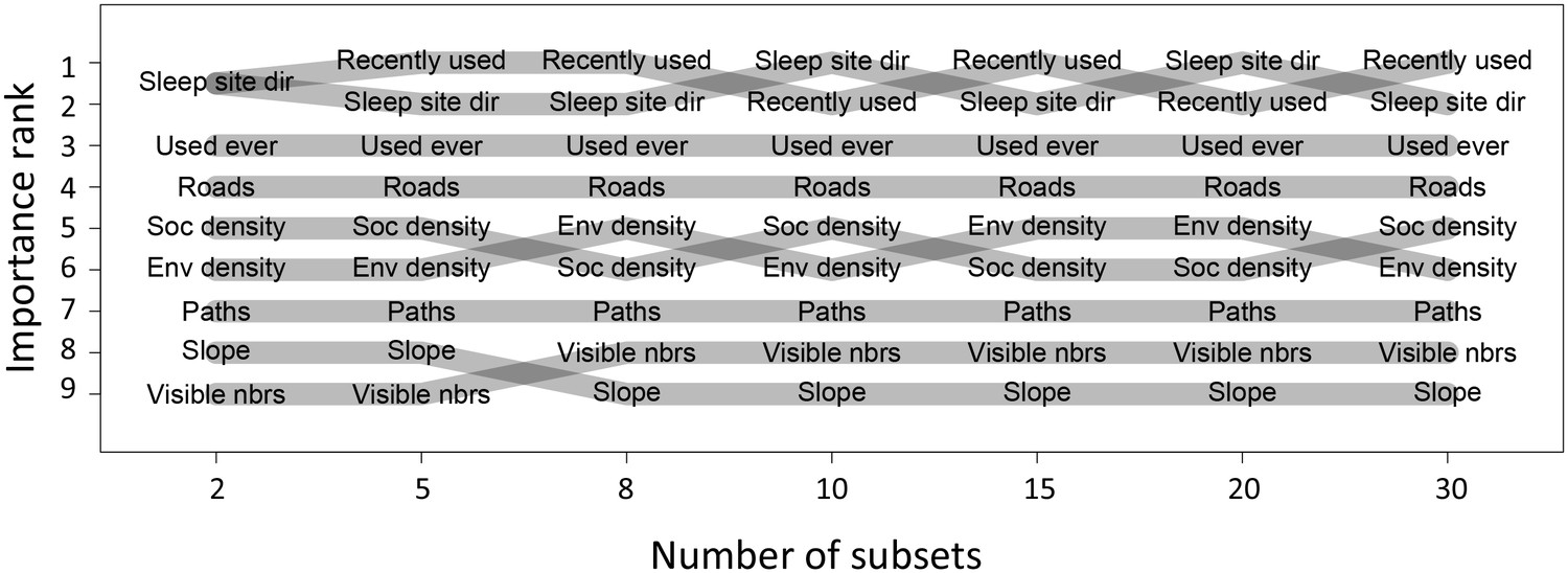
Relative importance ranks of habitat and social features do not depend on number of subsets used.
Plot shows the relative importance rank (features ranked by AIC weights, y-axis) based on multi-model inference across a range of numbers of subsets used (x-axis). Although the exact values of the AIC weights depend on the number of subsets used, their ranking is minimally changed across a wide range of possible numbers of subsets (few, and only local, swaps between feature ranks). This indicates that the rank order of features is relatively robust to the number of subsets used.
Appendix 1—figure 10
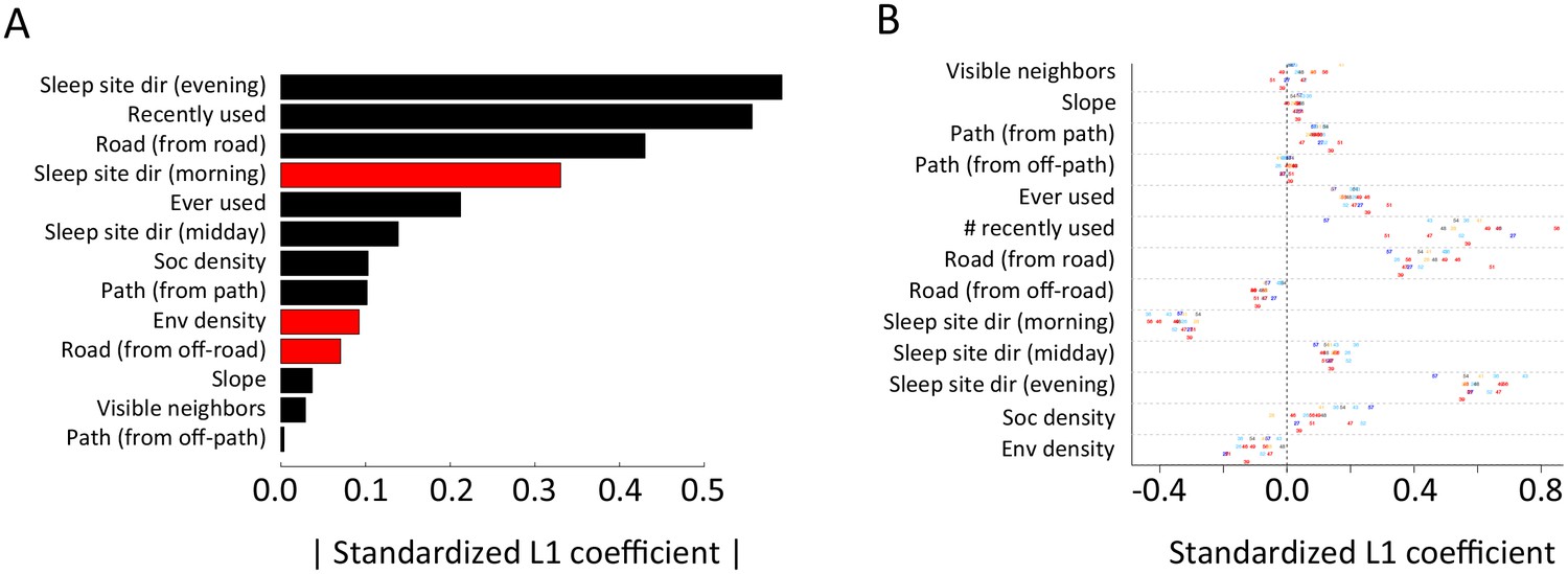
Alternative analysis: L1 regularization results.
Model coefficients for step selection models fit using L1 regularization as an alternative to multi-model inference. (A) Bars represent median L1 standardized coefficients (across all individuals) for each predictor. The length of each bar represents the absolute value of the coefficient, and the color represents the sign of the coefficient (black bars indicate positive coefficients, red bars indicate negative coefficients). (B) L1 standardized coefficients for each individual baboon (x-axis) for each predictor (y-axis). Data markers indicate collar numbers for each baboon.
Appendix 1—figure 11
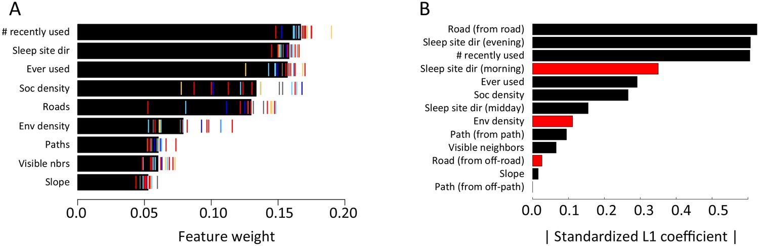
Step selection results for an alternative step size of R = 10 m.
(A) Results of multi-model inference (compare to Figure 1C). (B) Results of fitting using L1 regularization (compare to Appendix 1—figure 10).
Appendix 1—figure 12

The interplay between habitat and social features in shaping individual movement decisions: lower-ranked features.
An extension of the analysis shown in Figure 3, showing the probability (y-axis) that a baboon chose a given location (location 1) over an alternative location (location 2) as a function the number of baboons to have recently (within the past 4.5 min) occupied each of the two locations (x-axis), under various differences in other habitat and social features. These other features include: (A) habitat / vegetation density, (B–C) animal paths, (D) social density, (E) visible neighbors, and (F) elevation difference. In panels A, D, E, and F, colored lines represent data from various ranges of the difference in the value of the associated feature between the two locations. In panels B–C, colored lines represent different possible situations, analogous to those shown in Figure 3B–C.
Appendix 1—figure 13
The interplay between habitat and social features in shaping individual movement decisions: alternative step size, R = 10 m.
Analysis is the same as in Figure 3 (panels A–F) and Appendix 1—figure 12 (panels G–L), but using a step size of 10 m instead of the 5 m step size used in the main analysis. Results are qualitatively the same as for the R = 5 m case, indicating the robustness of the analysis to the exact step size used.
Appendix 1—figure 14
Visualizing the preference landscape underlying individual movement decisions: another example.
Plots are as in Figure 2, but a different example is shown (a case where the focal baboon started on a road).
Appendix 1—figure 15
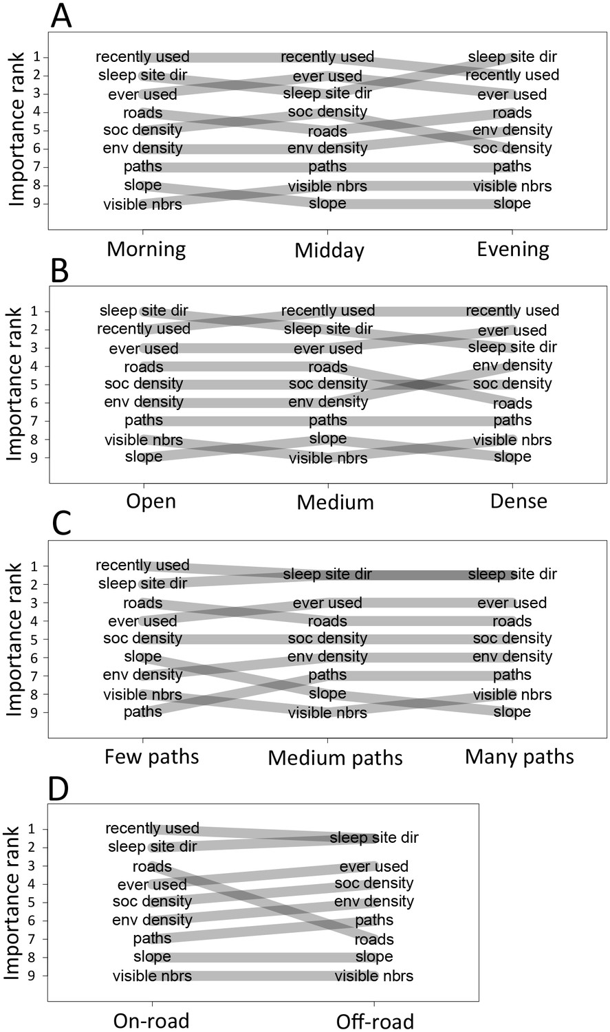
The priorities governing individual decisions vary as a function of context.
Plots show the importance ranks (ranks of AIC weights) of the different features in step selection models fit using data from each context. (A) Models fit for morning, midday, and evening data show that the relative importance rank (ranked AIC weight) of the sleep site direction (sleep site dir) and of roads decreases in the midday, while the relative importance rank of social density (how many other baboons are within a 4.25 m radius of a potential location) increases. (B) Models for different habitat densities show that, in particularly dense environments, the habitat / vegetation density (env density) feature becomes more important, while the sleep site direction (sleep site dir) and roads decrease in relative importance. The environment density of the group is defined as the average density inside the troop’s convex hull, and 'open', 'medium', and 'dense' categories represent the bottom, middle, and upper thirds of observed group habitat densities. (C) Models for different path densities show that, when the group is in an area with many paths, the relative importance of path-following increases, whereas the importance of ground slope increases when there are fewer paths. Path density was computed as the fraction of the area within the group’s convex hull that was located on a path. (D) Models for when the group was near a road (convex hull of the group overlapped a road) show high importance of roads, whereas when off a road, roads lose importance in predicting individual decisions.
Appendix 1—figure 16
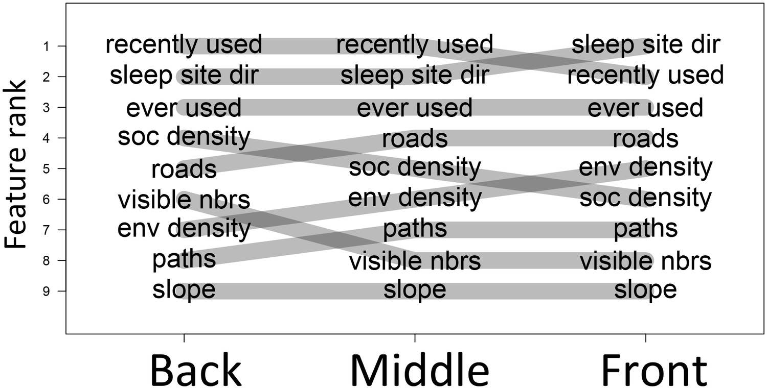
The priorities governing individual decisions vary as a function of an individual’s current position within the group.
In particular, for baboons at the front of the group, habitat features such as environment density (env density) and sleep site direction (sleep site dir) increase in relative importance, at the expense of social features such as how many baboons are within a 4.25 m radius of a potential location (soc density) and how many other baboons had previously occupied a location within the past 4.5 min (recently used).
Appendix 1—figure 17
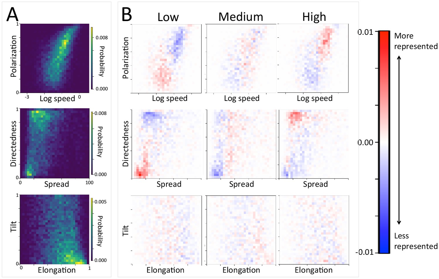
The density of paths in an area shapes group-level structure and movement dynamics.
(A) Two-dimensional histograms of group level properties across all data. Lighter areas indicate group configurations that are more likely to occur in the data. (B) Difference between the distributions within a given context (left column: low path density; middle column: medium path density; right column: high path density) and the overall distribution across all data. Redder areas represent group configurations that are over-represented within a given context (relative to the rest of the data), and bluer areas represent under-represented configurations. The path density was defined as the fraction of the area within the convex hull of the group that was on a path. In areas of high path density, the group tends to move faster, and in a more directed fashion. See Figure 4 and Supplementary methods for descriptions of how group-level properties were computed. See also Figure 6 and Appendix 1—figure 21.
Appendix 1—figure 18
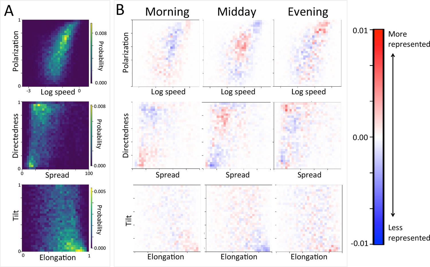
Group-level structure and movement dynamics changes as a function of time of day.
(A) Two-dimensional histograms of group level properties across all data. Lighter areas indicate group configurations that are more likely to occur in the data. (B) Difference between the distributions at different times of day (left column: morning; middle column: midday; right column: evening) and the overall distribution across all data. Redder areas represent group configurations that are over-represented within a given context (relative to the rest of the data), and bluer areas represent under-represented configurations. See Figure 4 and Supplementary methods for descriptions of how group-level properties were computed. See also Figure 6 and Appendix 1—figure 22.
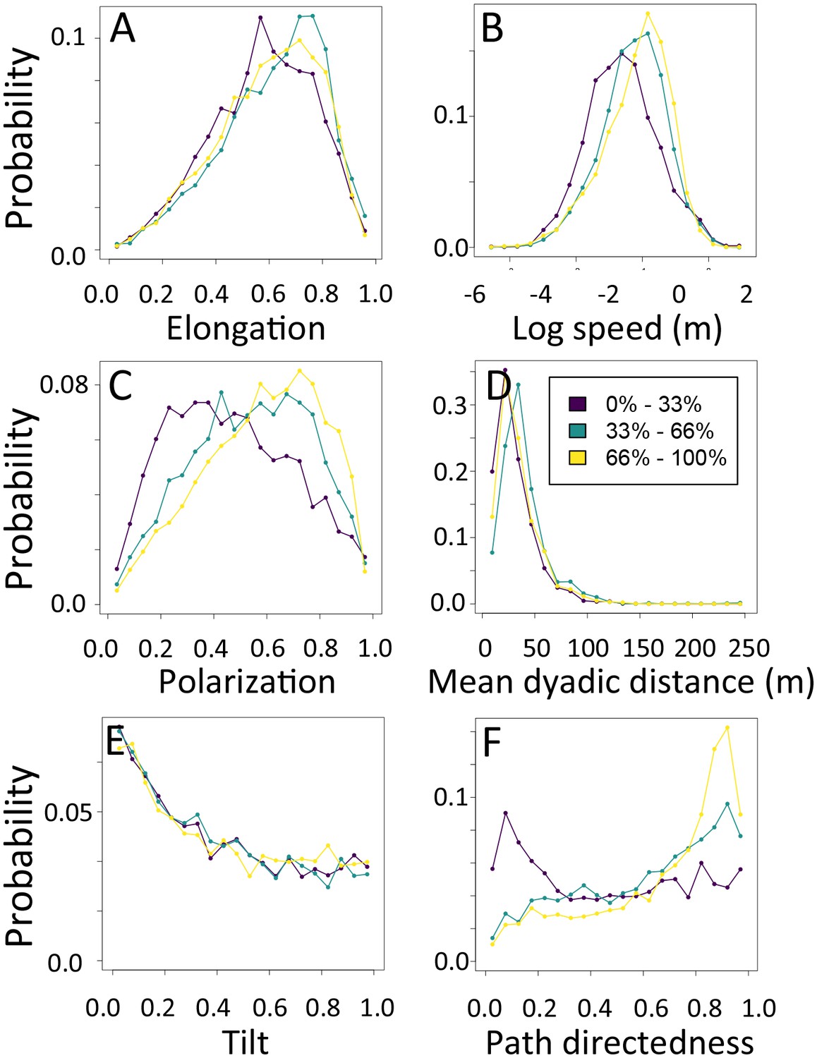
Appendix 1—figure 19
1-dimensional histograms of group-level properties as a function of environment density.
Distributions are shown for the highest third of environmental densities experienced by the group (light yellow), the middle third (green), and the bottom third (dark purple).
Appendix 1—figure 20

1-dimensional histograms of group-level properties as a function of whether the group was on a road (red) or off-road (black).
https://doi.org/10.7554/eLife.19505.031
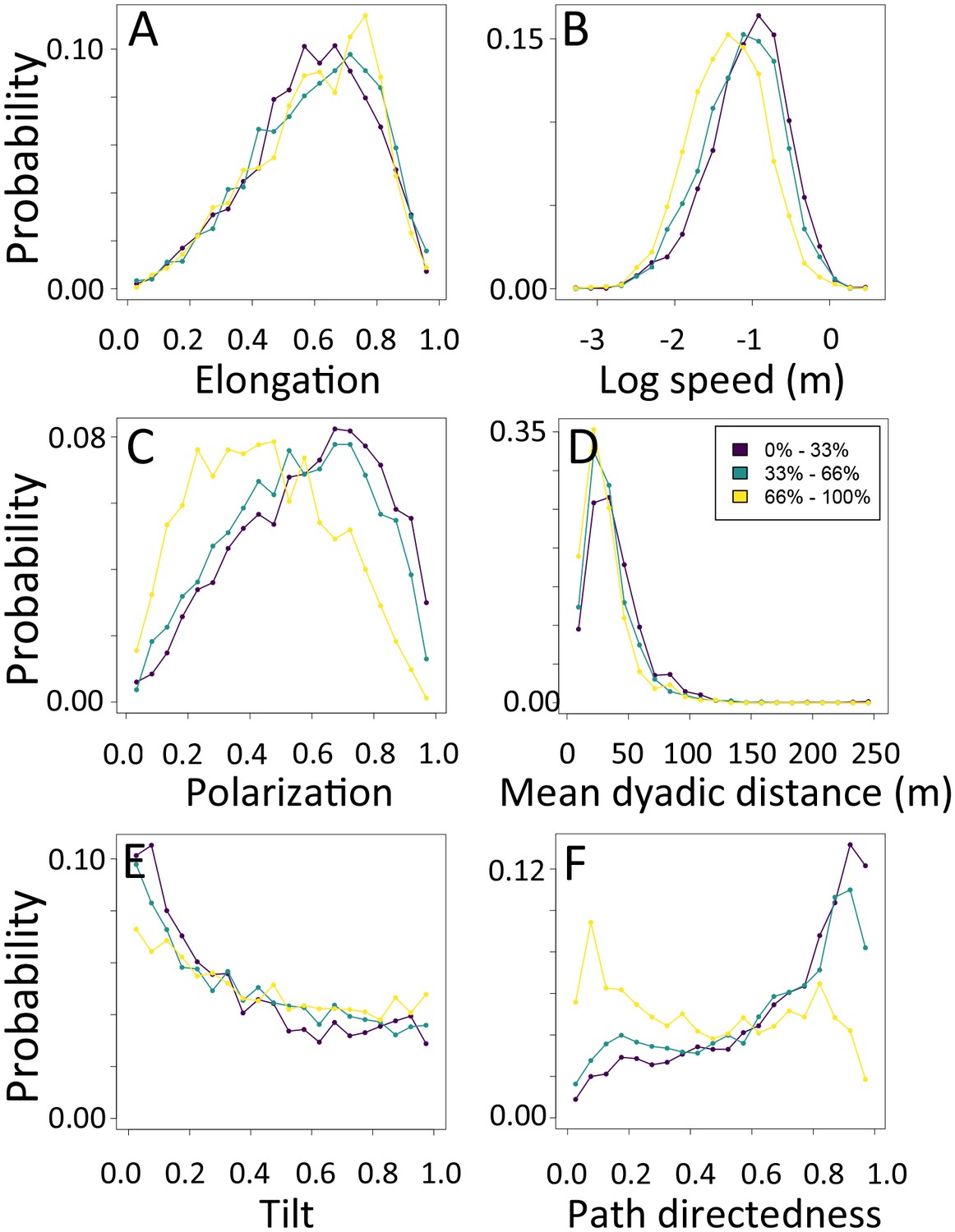
Appendix 1—figure 21
1-dimensional histograms of group-level properties as a function of path density.
Distributions are shown for the highest third of path densities experienced by the group (light yellow), the middle third (green), and the bottom third (dark purple).
Appendix 1—figure 22
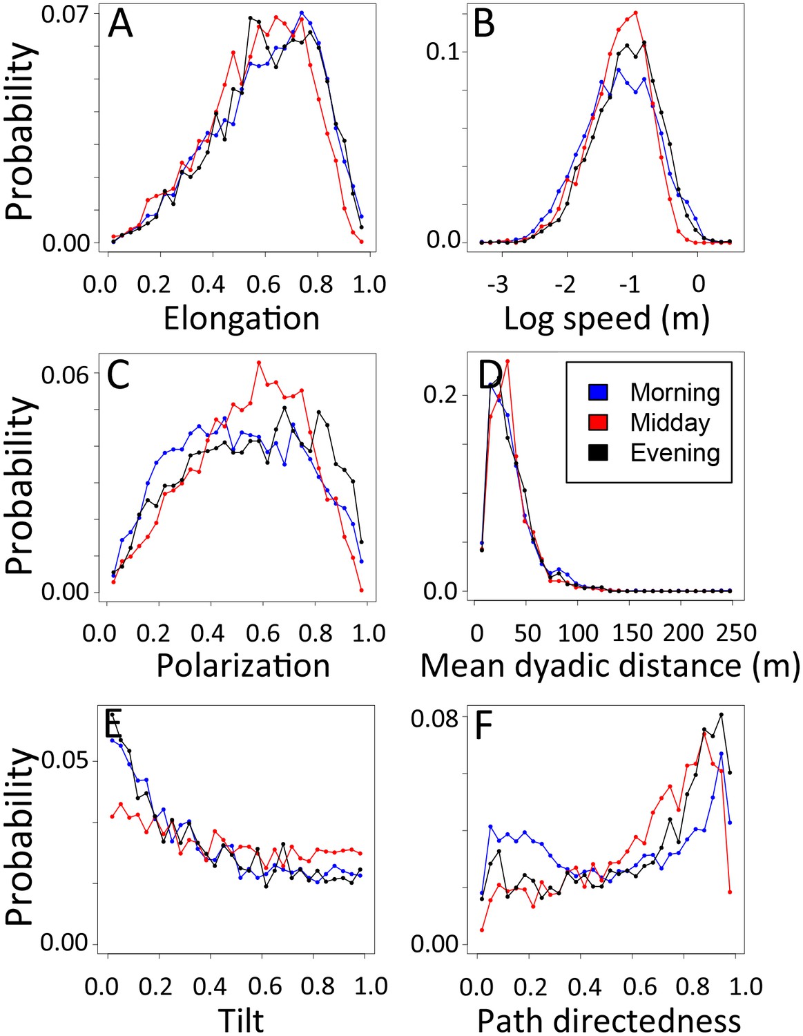
1-dimensional histograms of group-level properties as a function of time of day.
Distributions are shown for morning (blue), midday (red), and evening (black).
Appendix 1—figure 23

Baboon ranging patterns as a function of time of day (A: morning, B: midday, C: evening).
Colored points show locations of baboons throughout the first 14 days, and green lines show locations or roads. Baboons spent more time on roads in the morning (12.1%) and evening (12.1%) compared to during the midday period (7.5%).
Videos
Video 1
Animation of 3-dimensional habitat reconstruction (point cloud data).
https://doi.org/10.7554/eLife.19505.004
Video 2
Example of baboon trajectories overlaid on 3-dimensional habitat reconstruction.
Each point shows the movement of a single baboon within the troop, with color indicating the baboon’s age and sex (red: adult female, dark blue: adult male, orange: subadult female, light blue: subadult male, gray: juvenile male).
Tables
Table 1
Features (predictor variables) used in conditional logistic regression models to predict baboon movement decisions.
| Feature | Description | Type |
|---|---|---|
| Environment density | Fraction of non-ground (vegetated) area within a 2.5 m* radius of a potential location | Habitat Feature |
| Social density | Fraction of all troop mates within a 4.25 m* radius of a potential location | Social Feature |
| Sleep site direction | Direction of a potential location relative to the sleep site, ranges from −1 (directly away) to 1 (directly toward), fit as interaction with time of day | Habitat Feature |
| Roads | Whether a potential location is on a road (1) or not (0). Fit as an interaction with whether the baboon’s previous location was on a road | Habitat Feature |
| Recently-used space | Number of other baboons (not including focal individual) that have occupied a potential location within the past 4.5 min* | Social Feature |
| Ever-used space | Whether a potential location was ever occupied by another baboon (not including focal individual) across the entire dataset | Both |
| Animal paths | Whether a potential location is on an animal path (1) or not (0), fit as interaction with whether baboon’s previous location was on a path | Habitat Feature |
| Visible neighbors | Fraction of other group members visible from a potential location (i.e. direct line-of-sight does not pass through any vegetated areas) | Social Feature |
| Slope | Change in elevation to a potential location from the baboon’s previous location | Habitat Feature |
-
*Spatial and temporal scales were determined using maximum likelihood in a preliminary analysis. See Supplementary methods and Appendix 1—table 1 for further details.
Appendix 1—table 1
Features (predictor variables) used in conditional logistic regression models to predict baboon movement decisions.
| Feature | Description | Range | Considered as: |
|---|---|---|---|
| Environment density | Fraction of raster pixels containing non-ground points within a specified radius (R = 2.5 m) from the potential location (a proxy for vegetation density) | [0, 1] | Habitat Feature |
| Social density | Fraction of baboons currently tracked within a specified radius (Rsoc = 4.25 m) of the potential location | [0, 1] | Social Feature |
| Sleep site direction | The dot product of the direction vector from the current location to the potential location and the vector from the current location to the sleep site location. This quantity ranges from −1 (potential step is in the direct opposite direction from the sleep site) to 1 (potential step is directly toward the sleep site). The influence of the sleep site is expected to vary with time of day, therefore it is fit as an interaction with time of day, yielding three parameters. Times of day included Morning (9 am–12 pm), Midday (12–3 pm), and Evening (3–6 pm) | [−1, 1] | Habitat Feature |
| Roads | A binary predictor indicating whether the potential location is on a road or not. The influence of roads is expected to vary with whether an individual is currently on the road or not, therefore it is fit as an interaction with whether the baboon’s current location is on a road (also a binary value), yielding two parameters | {0, 1} | Habitat Feature |
| Recently-used space | An integer indicating how many other baboons (not including the focal individual) have recently (within the past 4.5 min) occupied the potential location, where a baboon is considered to be 'occupying a location' if its position is within 1 m of that location | {0, …, N} | Social Feature |
| Ever-used space | A binary variable that is defined as 1 if the location, was ever occupied by another baboon (not the focal baboon) throughout the entire dataset, (past, present, and future) | {0, 1} | Both |
| Animal paths | A binary variable indicating whether a potential location is on an animal path (1) or not (0). It is fit as an interaction with whether the baboon’s current location is on a path (also a binary value), yielding two parameters | {0, 1} | Habitat feature |
| Visible neighbors | A continuous variable that indicates the fraction of other group members that are visible from a given location at the time of the step. Group members were defined as visible if a line drawn from the potential location to their location at the relevant time does not pass through any raster cells containing non-ground points. | [0, 1] | Social feature |
| Slope | The change in elevation (in meters) from the starting location to a potential location | (−∞, ∞) | Habitat feature |
Download links
A two-part list of links to download the article, or parts of the article, in various formats.
Downloads (link to download the article as PDF)
Open citations (links to open the citations from this article in various online reference manager services)
Cite this article (links to download the citations from this article in formats compatible with various reference manager tools)
Habitat and social factors shape individual decisions and emergent group structure during baboon collective movement
eLife 6:e19505.
https://doi.org/10.7554/eLife.19505


