Naked mole-rat mortality rates defy Gompertzian laws by not increasing with age
Figures
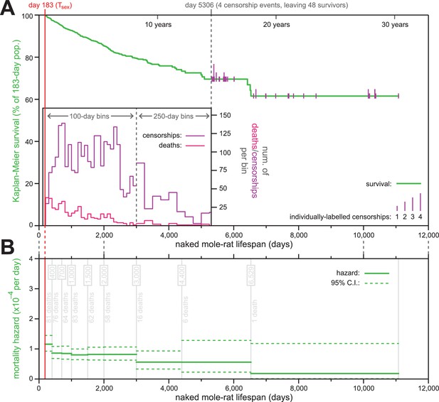
The mortality hazard of naked mole-rats failed to increase for at least 18 years.
(A) Kaplan-Meier survival curve for naked mole-rats (green) after reaching reproductive maturity (Tsex; 6 months from birth; 183 days; red). The surviving population size drops below 50 at day 5306 (of 52 animals surviving to that day, four are censored: grey). After that, censorship events are indicated as vertical ticks (purple), the size of which is proportional to the number of animals censored at each day-of-life. Before day 5306, the distributions of censorship events and death events are depicted as histograms (purple and pink, respectively), in either 100 day or 250 day bins. There were a total of 444 death events and 2803 censorship events after day 183 and prior to day 5306. (B) Mortality-hazard estimates (solid green) with 95% confidence intervals (dotted green) across the observed naked mole-rat lifespan. Estimates were calculated across time intervals of increasing size (demarked by grey lines) to compensate for decreasing accuracy-per-unit-time as the population size decreased. The number of observed deaths per bin is indicated in grey.
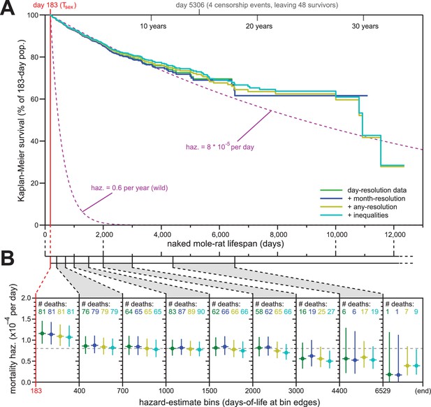
Addition of previously excluded, low-resolution lifespan data did not modify the apparent lifespan demographics of H. glaber.
(A) Repeated calculation of Kaplan-Meier survival, using the original data from Figure 1 (green) and iteratively adding month-resolution data (navy), less-than-month-resolution data (yellow), and inequality-derived data (cyan; see Materials and methods for further descriptions). Expected survivals from Tsex (purple) using either our consistent estimate for mortality hazard (8 * 10−5 per day) or an estimate from Hochberg (Hochberg et al., 2016) for H. glaber survival in the wild (0.6 per year). (B) Hazard estimates across each of the lifespan bins from Figure 1B, calculated for each of the expanded data sets, as described and colored in panel (A). Vertical bars indicate 95% confidence intervals. The number of observed deaths per bin is indicated at the top of each panel, colored according to the data set. Dotted grey line indicates 8 * 10−5 deaths/day.
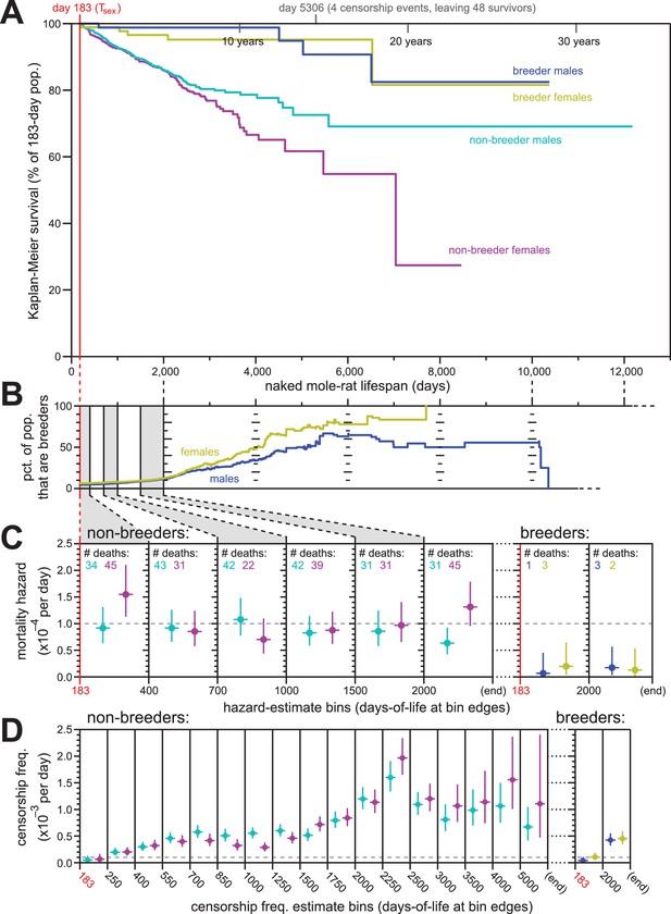
Breeding and non-breeding males and females exhibited non-increasing mortal hazard as a function of age.
(A) Repeated calculation of Kaplan-Meier survival, splitting the data from Figure 1 into four categories: male breeders (navy), female breeders, (yellow), male non-breeders (cyan), and female non-breeders (purple). (B) The percentage of the population recorded as being breeders as a function of age, for females (yellow) and males (navy). (C) Hazard estimates for the indicated lifespan bins (x-axis), calculated separately for non-breeders (left) versus breeders (right), and males versus females (colored as in panel A). Grey dashed line indicates 1/10,000 per day. (D) Estimates of the probability of being censored for the indicated lifespan bins (x-axis), displayed separately for non-breeders versus breeders, males versus females, as in panel (C). Grey dashed line again indicates 1/10,000 per day.
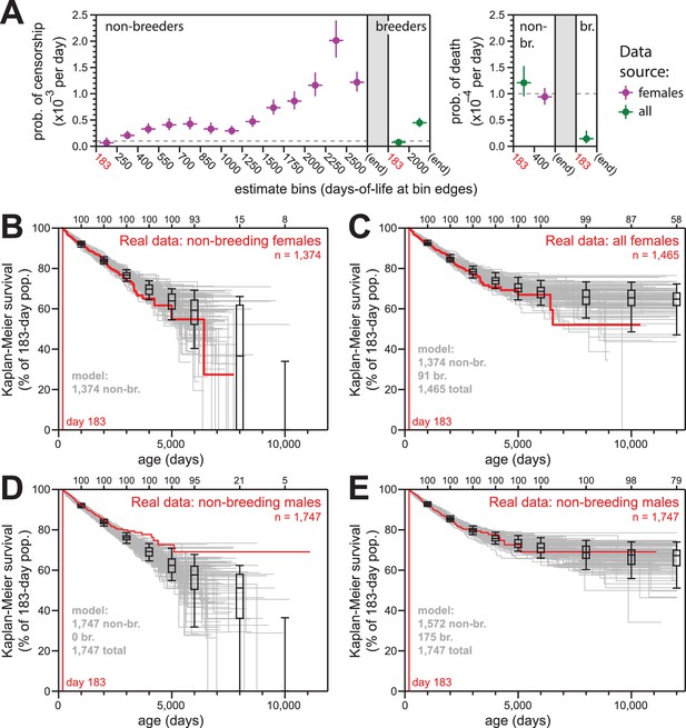
Simulations of naked mole-rat survival, run assuming constant mortality hazard, re-capitulated the observed data when breeders and non-breeders were appropriately balanced.
(A) The model applied here: per-day probabilities of censorship and death for non-breeders and breeders. Separate probabilities were assigned to each age bin indicated on the x-axes. Colors indicate the source data for the estimate used in the model (purple for females; green for both sexes), and error bars indicate 95% confidence intervals for the estimates used to build the model. (B) Kaplan-Meier plots for 100 simulations of populations with 1374 non-breeders (grey) versus the true plot for the 1374 non-breeding females (red). Box-and-whiskers indicate the median, quartile, and 5th/95th percentile survival values for simulated populations that had not terminated due to censorship (i.e. 0%-survival populations were included); number of included simulations is indicated along the top axis. (C) Kaplan-Meier plots for 100 simulations of populations with 1374 non-breeders and 91 breeders (grey) versus the true plot for the 1374 non-breeding and 91 breeding females (red). Box-and-whiskers as in panel (B). (D) Kaplan-Meier plots for 100 simulations of populations with 1747 non-breeders (grey) versus the true plot for the 1747 recorded-as-non-breeding males (red). Box-and-whiskers as in panel (B). (E) Kaplan-Meier plots for 100 simulations of populations with 1747 individuals, split into 1572 non-breeders and 175 breeders (grey) versus the true plot for the 1747 recorded-as-non-breeding males (red). Box-and-whiskers as in panel (B).
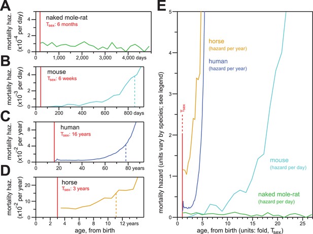
In contrast to the mortality hazards of other mammals, which increased with chronological age, the mortality hazard of naked mole-rats remained constant.
(A–D) Age-specific mortality hazard for naked mole-rats (A; green), calculated for 200 day intervals; for mice (B; cyan), calculated for 50 day intervals using the control-mouse survival data reported by Miller (Miller et al., 2014); for human females (C; navy), by year, as reported for the 1900 birth cohort by Bell and Miller (Bell and Miller, 2005); and for horses (D; orange), by year, calculated from life insurance tables reported by Valgren (Valgren, 1945). Calculations begin after Tsex for each species (red). (E) Hazard plots from panels A-D, re-scaled on the x-axis to the time it takes each organism to reach Tsex from birth.
Additional files
-
Source code 1
Supplemental Python Script.
A simulator for breeder/non-breeder population survival simulation, implementing the method described for Figure 4 and with output formatted as in Supplementary file 3–6. Run the script using python (recommended: Python 2.7.13) with no additional arguments for user-level documentation. Read the script (provided as a text document) for developer-level documentation.
- https://doi.org/10.7554/eLife.31157.007
-
Supplementary file 1
Animal-by-animal lifespan and annotation data.
This is a comma-separated text file with 11 columns. Each row in the file contains data for one animal. Column 1 (‘IsDead’) indicates whether the animal was dead or alive at the time these data were compiled. Column 2 (‘AnimalID’) is a unique identifier for each animal (to facilitate reference/discussion). Column 3 (‘BirthDate’) is the date-of-birth according to our records (varying degrees of resolution: month/day/year in the ideal case). Column 4 (‘Sex’) indicates both the sex of the animal (‘M’/'F’ for male/female) and breeding status (addition of a ‘B’ when an individual was known to be a breeder), as documented in our historical records. Column 5 (‘Notes’) include information on the death or censorship event (classified as described in the previous paragraph). Column 6 (‘DeathDate’) indicates, for dead/censored animals, the date of that event. It is empty if the animal were still alive at the time of data compilation. Column 7 (‘DataDate’) indicates the date on which data for that animal was compiled. If the animal were still alive, that date is used as the date-of-censorship. Column 8 (‘ValidBirth’) indicates whether the birth was single-day-resolution, that is sufficient for inclusion in the analysis set for Figure 1 (‘Y’/'N’ for yes/no). Column 9 (‘ValidDeathCen’) gives the same indication for the date of death or censorship. Column 10 (‘Censored’) indicates the classification of death-versus-censorship (‘Y’ indicates censorship). Column 11 (‘Lifespan(days)”) gives the number of days of life for all animals with ‘Y’ values (indicating single-day-resolution) in both columns 8 and 9.
- https://doi.org/10.7554/eLife.31157.008
-
Supplementary file 2
Parameters for demographic simulations.
This is a comma-separated text file with 5 columns. Column 1 (‘DeathOrCen’) indicates if the given row provides hazard for either death (‘D’) or censorship (‘C’) events. Column 2 (‘Breeder’) indicates whether the row provides hazard for breeders (yes; ‘Y’) or non-breeders (no; ‘N’). Column 3 (‘Start’) indicates the first day to which the hazard from that row should be applied. Column 4 (‘Finish’) indicates the day on which the hazard from that row should stop being applied (or ‘(end)’ if the value should be applied indefinitely). Column 5 (‘Hazard/day’) gives the per-day probability (hazard) of the event described in column 1 occurring for the animal described in column 2.
- https://doi.org/10.7554/eLife.31157.009
-
Supplementary file 3
Simulations from Figure 4B.
These simulations were run as described in Methods, with a starting population of 1374 non-breeders. One hundred simulations were run. This is a comma-separated text file with 4 columns. Each row in the file contains data for one simulated animal. Column 1 (‘Sim’) indicates which of the 100 simulations the animal was a part. Column 2 (‘Br’) indicates breeding status (‘Y’ for breeders, ‘N’ for non-breeders). Column 3 (‘Ls’) indicates the lifespan of the animal, in days. Column 4 (‘Cen’) indicates whether the animal’s lifespan ended with censorship or death (‘Y’ for censorship, ‘N’ for death).
- https://doi.org/10.7554/eLife.31157.010
-
Supplementary file 4
Simulations from Figure 4C.
These simulations were run as described in Methods, with a starting population of 91 breeders and 1374 non-breeders. One hundred simulations were run. This is a comma-separated text file, formatted as described for Supplementary file 3.
- https://doi.org/10.7554/eLife.31157.011
-
Supplementary file 5
Simulations from Figure 4D.
These simulations were run as described in Methods, with a starting population of 1747 non-breeders. One hundred simulations were run. This is a comma-separated text file, formatted as described for Supplementary file 3.
- https://doi.org/10.7554/eLife.31157.012
-
Supplementary file 6
Simulations from Figure 4E.
These simulations were run as described in Methods, with a starting population of 175 breeders and 1572 non-breeders. One hundred simulations were run. This is a comma-separated text file, formatted as described for Supplementary file 3.
- https://doi.org/10.7554/eLife.31157.013
-
Transparent reporting form
- https://doi.org/10.7554/eLife.31157.014


