Ant colonies maintain social homeostasis in the face of decreased density
- Penn State University, United States
- Georgetown University, United States
Figures
Figure 1 with 4 supplements
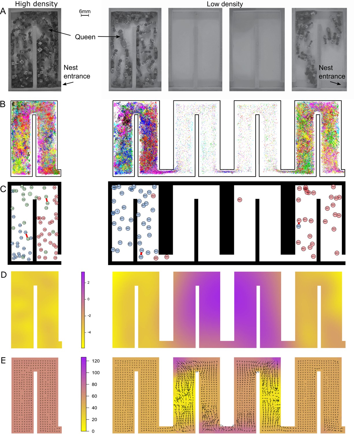
At low density, colonies exhibit dramatically different movement patterns in the center part of the nest that result in faster travel between groups.
(A) Still images from the videos that were used to track ants in colony 1 in high- (one chamber) and low-density (four chambers) environments. (B) Tracking data for all ants in colony 1. (C) Still images from the animations visualizing ant identity (each labeled polygon represents a specific ant), spatial group (color of each polygon) and trophallaxis (red line between two polygons) in colony 1. For people with impaired color vision, geometric shapes were added to distinguish colors (pink = circle, blue = hexagon, green = octagon). (D) Motility surface plot illustrating the spatial variation in the average movement rates of colony. At low density, the faster movement rates in the middle chambers suggest that workers use this part of the chambers as a ‘highway’ between the entrance and the back of the nest. (E) Potential surface plot revealing the directional force that acts on an ant when she moves through the nest. Lower values indicate a downhill slope that causes an acceleration. Accordingly, higher values represent an uphill slope, that is deceleration.
Figure 1—figure supplement 1
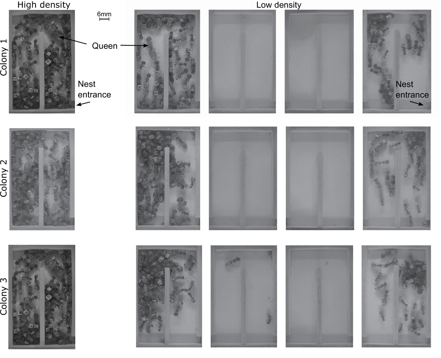
Screenshots taken from videos of high and low density colonies at time zero.
https://doi.org/10.7554/eLife.38473.003
Figure 1—figure supplement 2
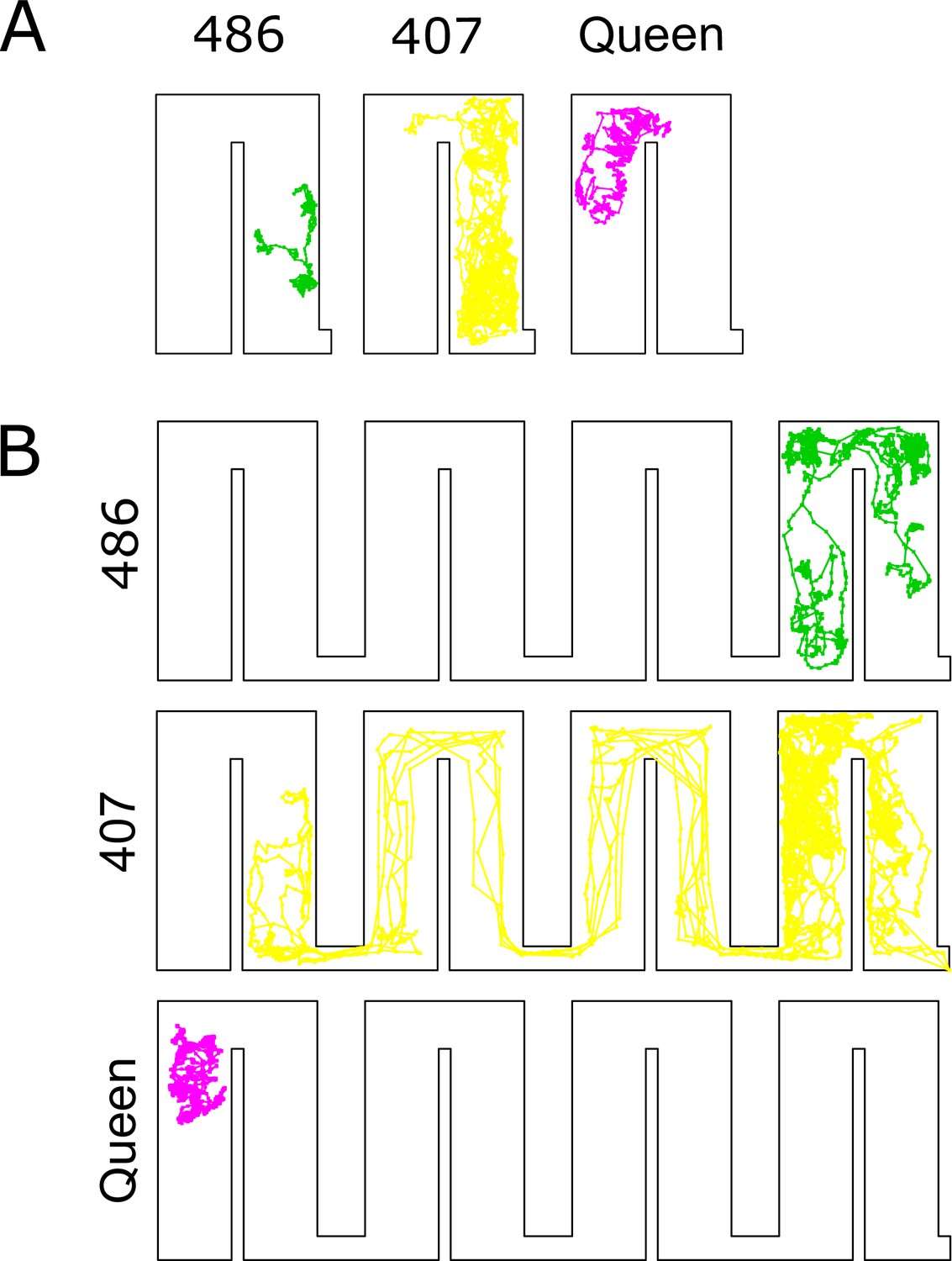
Individual movement trajectories of a few selected individuals for colony 1 in high (A) and low-density (B) periods.
Workers are labeled with numbers.
Figure 1—figure supplement 3
Motility plots illustrating the spatial variation in the average movement rates for all colonies in the different nest chambers during high- and low-density periods.
All colonies show a much higher average movement rate in the two middle chambers.
Figure 1—figure supplement 4

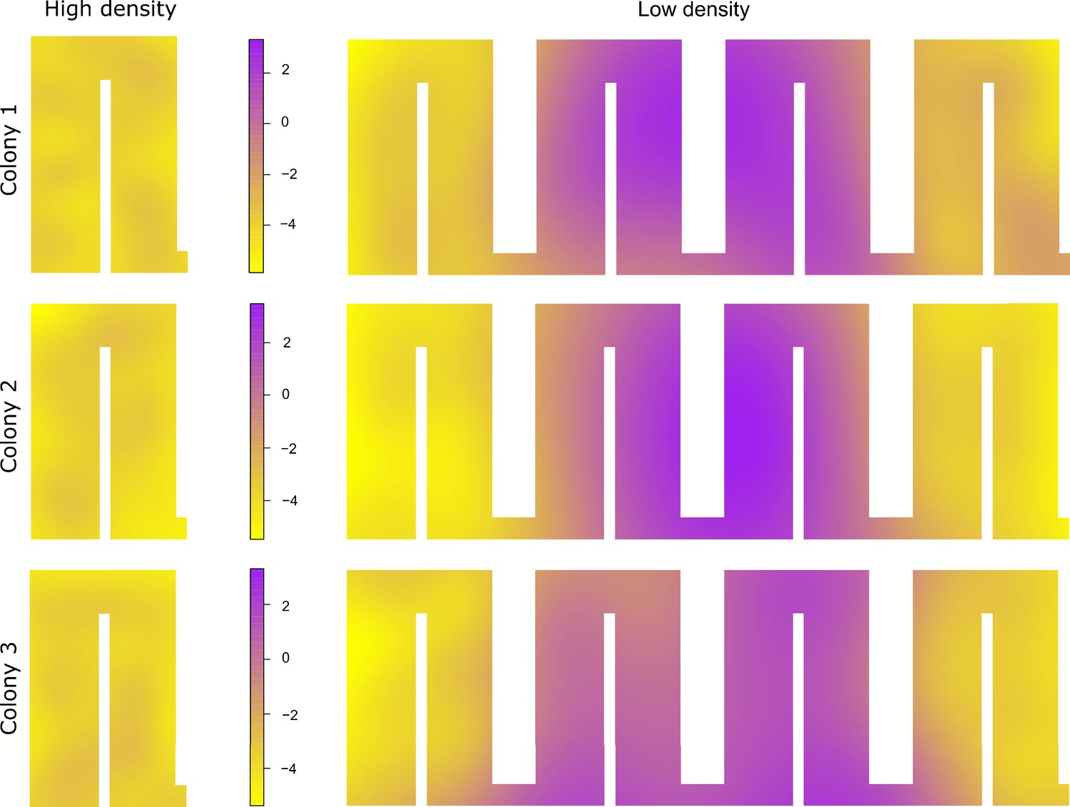
Potential surface plots for all colonies during high- and low-density period.
Higher values indicate that individuals slow down, whereas lower values suggest that ants accelerate. Some general patterns are maintained in all colonies, with potential surfaces pushing ants to turn quickly around corners. Differences in the estimated levels of the potential surface in the end chambers are caused by observing different numbers of ants moving from right to left vs. from left to right in the 4 hr observation window.
Figure 2 with 6 supplements
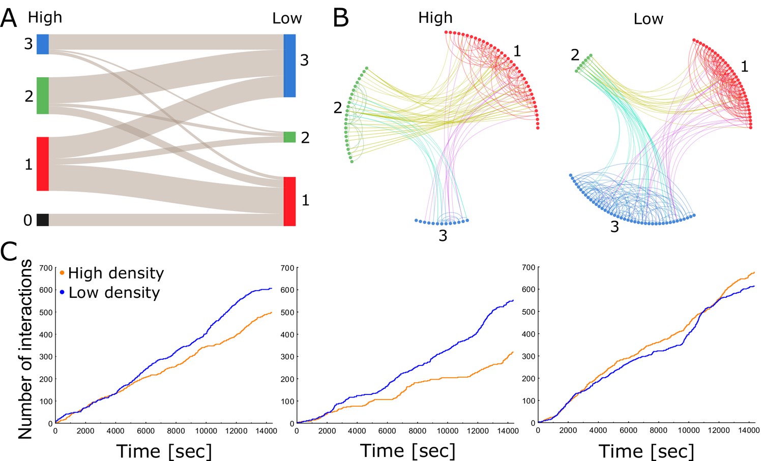
Each colony consists of a network of tightly knit spatial groups that exhibits remarkable resilience to changes in density.
(A) The colored columns depict the different spatial groups identified by the clustering algorithm in the high- and low-density treatments of colony 2. Low numbers represent a closer position to the entrance. The gray lines between these groups visualize that the ants preferred to remain in a similar spatial position relative to each other when nest size was increased. (B) Trophallaxis networks of colony 2 before (high density) and after nest expansion (low density). Each node represents an ant in the network with color indicating its spatial group. Groups are arranged in a circle and sorted numerically on the basis of their average distance to the entrance. Specifically, group 1 was closest to the entrance and group 3 furthest away. (C) Cumulative number of interactions (food sharing events) over time during high- and low-density periods for colonies 1, 2 and 3 (from left to right).
Figure 2—figure supplement 1

The colored columns depict the different spatial groups identified by the clustering algorithm during the high- and low-density periods for colonies 1, 2 and 3 (from left to right).
Low numbers represent a closer position to the entrance. The gray lines between these groups indicate that the ants preferred to remain in a similar spatial position relative to each other when nest size was increased. Please note that there was no spatial group 0 (ants that were outside during the entire observation period) during the low-density period. The black column in the low-density period instead represents ants that died between the high and low-density periods (colony 2 had zero deaths).
Figure 2—figure supplement 2
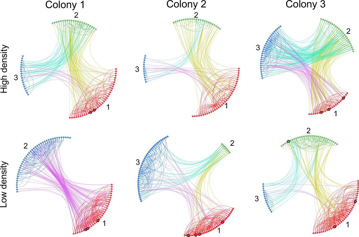
Trophallaxis networks of all colonies before (high density) and after nest expansion (low density).
Each node represents an ant in the network with color indicating its spatial group. Foragers are marked with black circles. Groups are arranged in a circle and sorted numerically on the basis of their average distance to the entrance. Specifically, group 1 was closest to the entrance and group 3 furthest away.
Figure 2—figure supplement 3

Location of trophallaxis (food sharing) events during the low- and high-density periods.
Each circle represents an interaction between two ants with color indicating spatial groups. Red, green and blue represent interactions within spatial groups 1, 2 and 3, respectively. Interactions between spatial groups are colored with cyan (green + blue), purple (red + blue) and yellow-green (red + green).
Figure 2—figure supplement 4

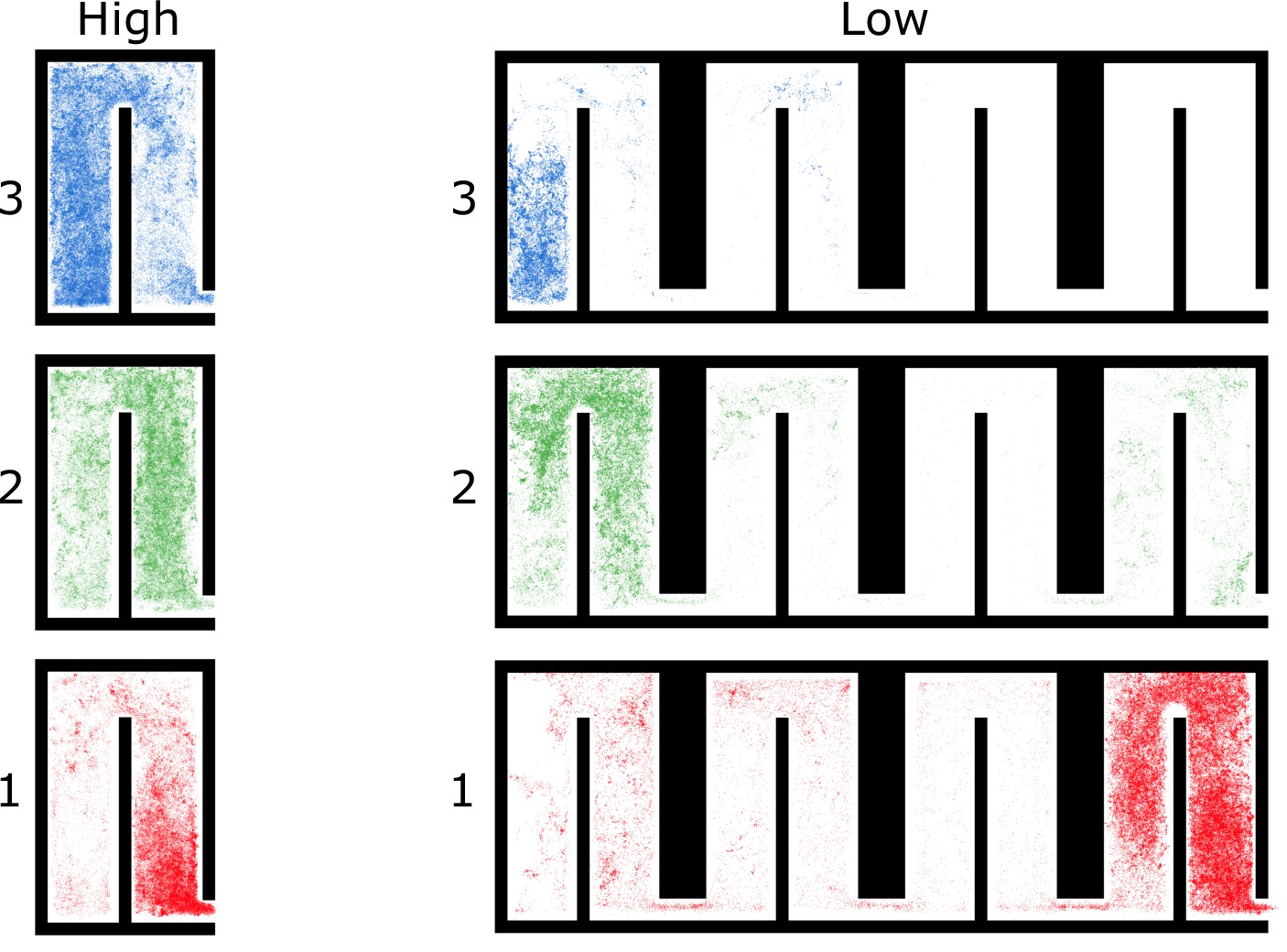
All locations of ants in colony 1 by spatial group and density treatment.
For each group, we plotted every location of every ant in the group over the 4 hr period. Please note that there are three groups during the high-density period and only two groups during the low-density period.
Figure 2—figure supplement 5

All locations of ants in colony 2 by spatial group and density treatment.
For each group, we plotted every location of every ant in the group over the 4 hr period.
Figure 2—figure supplement 6
All locations of ants in colony 3 by spatial group and density treatment.
For each group, we plotted every location of every ant in the group over the 4 hr period.
Figure 3
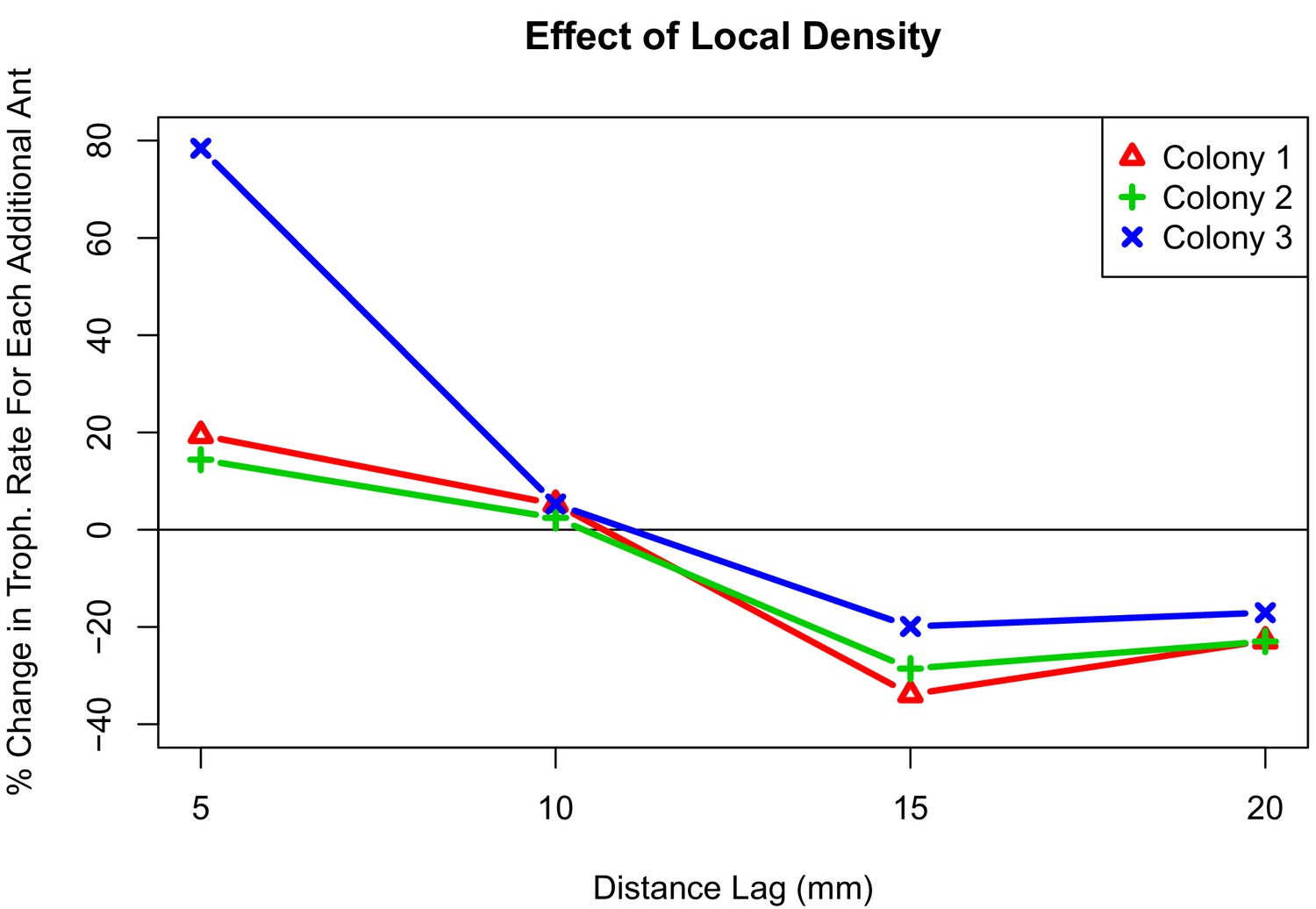
Interaction plot depicting the effect of local density on trophallaxis rate over a range of radii.
The values shown are the percent change in average rate of trophallaxis events when one additional ant is present at different distance lags. For all colonies, additional ants within 10 mm correlate with increased rate of trophallaxis events, while additional ants within 10 mm–20mm correlate with a decreased rate of trophallaxis events.
Figure 4
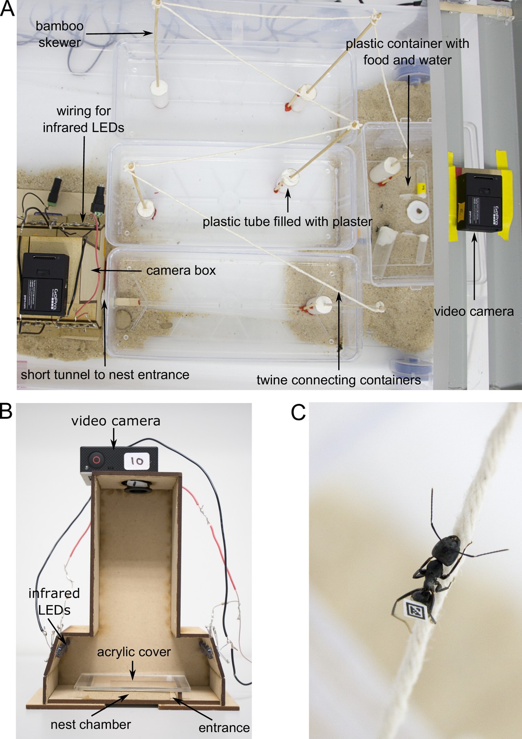
Experimental set-up.
(A) Overview of the foraging arena. (B) Camera box with side wall removed to show inner parts. (C) Worker walking over twine. Photos by Christoph Kurze.
Videos
Video 1
Animation for colony 1 depicting the combined tracking and trophallaxis during the low-density period for about 1 hr of data.
Ants are represented as circles with their identity (numbers identify workers, ‘Q’ represents the queen). Food sharing is visualized as a red line between two individuals. Circle color indicates spatial-group affiliation. Video runs at 10 times normal speed.
Tables
Table 1
Summary of the parameter estimates of a generalized linear model with Poisson distribution and log-link predicting the number of interactions that were initiated each second depending on treatment (high versus low density) and colony identity (1, 2 and 3).
Total sample size is 86,406. 14,401 observation points (one observation per second) per treatment and colony (14,401 × 2×3=86,406). CL, confidence limit.
| Level of effect | Estimate | Standard error | Wald stat. | Lower CL 95% | Upper CL 95% | p-value | |
|---|---|---|---|---|---|---|---|
| Intercept | −3.30 | 0.02 | 33538.95 | −3.34 | −3.27 | <0.0001 | |
| Colony | 1 | 0.04 | 0.03 | 1.97 | −0.01 | 0.08 | 0.16 |
| Colony | 2 | −0.23 | 0.03 | 71.58 | −0.28 | −0.18 | <0.0001 |
| Treatment | High | −0.11 | 0.02 | 36.34 | −0.14 | −0.07 | <0.0001 |
| Colony*Treatment | 1 | 0.01 | 0.03 | 0.12 | −0.04 | 0.06 | 0.73 |
| Colony*Treatment | 2 | −0.16 | 0.03 | 36.86 | −0.22 | −0.11 | <0.0001 |
-
Table 1—source code 1
R code for the pairwise comparison of the interaction terms colony by treatment presented in Table 1—source data 2.
- https://doi.org/10.7554/eLife.38473.016
-
Table 1—source data 1
The source data for the results presented in Table 1 and Table 1—source data 2.
- https://doi.org/10.7554/eLife.38473.017
-
Table 1—source data 2
Pairwise comparison of the colony by treatment interaction terms presented in Table 1.
- https://doi.org/10.7554/eLife.38473.018
Table 2
Results of a pair-based analysis of when ant pairs initiate trophallaxis.
We modeled trophallaxis initiations for each pair as coming from an inhomogeneous Poisson point process, where the rate of trophallaxis initiations depends on colony and local-density effects. We included effects for each colony and experimental condition (high or low), and also considered interactions between colony and the local density at 5 mm (n5), 10 mm (n10), 15 mm (n15), and 20 mm (n20).
| Estimate | Standard error | Z-value | p-value | |
|---|---|---|---|---|
| Colony 1 | −5.80 | 0.07 | −82.25 | <2e-16 |
| Colony 2 | −6.04 | 0.09 | −69.18 | <2e-16 |
| Colony 3 | −8.59 | 0.29 | −30.04 | <2e-16 |
| Treatment | −0.49 | 0.04 | −11.11 | <2e-16 |
| n5 | 0.18 | 0.04 | 4.08 | 4.60e-05 |
| n10 | 0.05 | 0.02 | 2.08 | 0.04 |
| n15 | −0.41 | 0.03 | −15.01 | <2e-16 |
| n20 | −0.26 | 0.02 | −10.57 | <2e-16 |
| col2:n5 | −0.04 | 0.07 | −0.62 | 0.5335 |
| col3:n5 | 0.40 | 0.07 | 5.98 | 2.30e-09 |
| col2:n10 | −0.03 | 0.04 | −0.69 | 0.49 |
| col2:n15 | 0.08 | 0.04 | 1.77 | 0.08 |
| col3:n15 | 0.19 | 0.03 | 5.84 | 5.29e-09 |
| col2:n20 | −0.002 | 0.04 | −0.06 | 0.96 |
| col3:n20 | 0.07 | 0.03 | 2.14 | 0.03 |
Additional files
-
Transparent reporting form
- https://doi.org/10.7554/eLife.38473.022
Download links
A two-part list of links to download the article, or parts of the article, in various formats.
Downloads (link to download the article as PDF)
Open citations (links to open the citations from this article in various online reference manager services)
Cite this article (links to download the citations from this article in formats compatible with various reference manager tools)
Ant colonies maintain social homeostasis in the face of decreased density
eLife 8:e38473.
https://doi.org/10.7554/eLife.38473


