Functional connectivity in human auditory networks and the origins of variation in the transmission of musical systems
- Aarhus University and The Royal Academy of Music, Denmark
- Norwegian University of Science and Technology, Norway
Figures
Figure 1
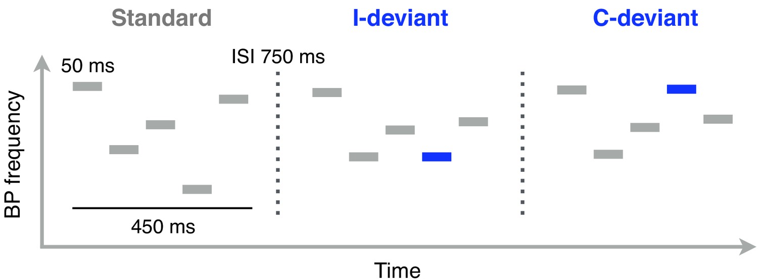
Schematic illustration of Bohlen-Pierce (BP) tone sequences used in the functional localizer task (auditory oddball).
Functional MRI scanning was performed while participants listened to these sequences. Each sequence consisted of 5 sinusoidal 50 ms tones separated by 50 ms of silence. The intersequence interval (ISI; the silent gap between the offset of one sequence and the onset of the next one) was 750 ms. Standard sequences (80% of trials) were randomly transposed at different registers. Deviant sequences featured a change in pitch interval (interval deviants, I-deviants; 10%) or melodic contour (contour deviants, C-deviants; 10%) of the fourth tone, relative to its position in standard sequences.
Figure 2

Schematic example of the formal measures used on signaling game data.
Tone and Contour entropy: A single entropy value (H) was computed for each tone sequence (Tone entropy) and the relative contour transform (Contour entropy) by using the Shannon entropy formula. These measures are different indicators of the complexity of a melodic signal. Asymmetry: we calculated asymmetry in Game 2 as the difference of the number of code changes introduced by the sender (S) and by the receiver (R) across all emotions, divided by the total number of code changes ((S–R)/(S+R)). This measure reflects the direction of information flow and ranges from −1 (the receiver adapts his mappings to the ones used by the sender) to 1 (viceversa). In Game 1, the sender never changes the signal-to-emotion mappings and asymmetry is −1 by design. Coordination: we computed coordination in Game 1 as the mean similarity (1-Hamming distance) between the signal (tone sequence or contour transform) used by the sender for a given emotion and the set of signals mapped by the receiver to the same emotion during the second half of the game (between-player measure). A mean value was computed across all five emotions. It represents the extent to which the sender and receiver shared their mappings at the end of the game and it ranges from 0 (different signaling system) to 1 (shared signaling system). Transmission: this measure was computed as the similarity of signals (tone sequences or contour transforms) mapped to the same emotion and used by senders of adjacent games (between-player measure). A mean value was computed across emotions. It ranges from 0 (the sender in game two reproduced a new signaling system) to 1 (the sender in game two faithfully transmitted the signaling system received in game 1). Innovation: this measure was calculated as the mean hamming distance (HD) between the signal (tone frequency or contour transform) mapped with the greatest frequency to a given emotion in the second half of Game 1 by the player as receiver and the signal reproduced with major frequency for the same emotion in Game 2 by the same player as sender (within-player measure). A mean value was computed across the five emotions, ranging from 0 to 1. Values close to one indicate that a significant number of changes were introduced in the signaling system by the participant. Interval compression ratio: The interval compression ratio (ICR) (Tierney et al., 2011) was calculated as the ratio between the mean absolute interval size (in macrotones) of a tone sequence randomly scrambled (N = 100), divided by the mean absolute interval size of the original sequence. A mean value was computed across the five emotions. Larger values indicate a bias towards smaller (proximal) intervals. Scripts to compute these measures are available at: https://doi.org/10.5061/dryad.2jj01c1 (folder ‘signaling games’).
Figure 3

Trial structure and experimental transmission design.
(a) Example of a trial from the signaling games played by participants in the second session of the study. The top and bottom rows show what senders and receivers saw on the screen, respectively. For the sender, the task was to compose an isochronous five-tone sequence to be used as a signal for the simple and compound emotions expressed by the image shown on the screen at the start of each trial. For the receiver, the task was to respond to that signal by guessing the image the sender had seen. The sender and the receiver converged over several trials on a shared mapping of signals (tone sequences) to meanings (emotions). Hand symbols indicate when the sender or the receiver had to produce a response. Feedback was provided to both players simultaneously, showing the face seen by the sender and the face selected by the receiver in a green frame (matching faces; correct) or in a red frame (mismatching faces; incorrect). Time flows from left to right. (b) Experimental transmission design in signaling games. The participant played as receiver (R) with a confederate of the experimenters playing as sender (S) in Game 1. Roles switched in Game 2.
Figure 4
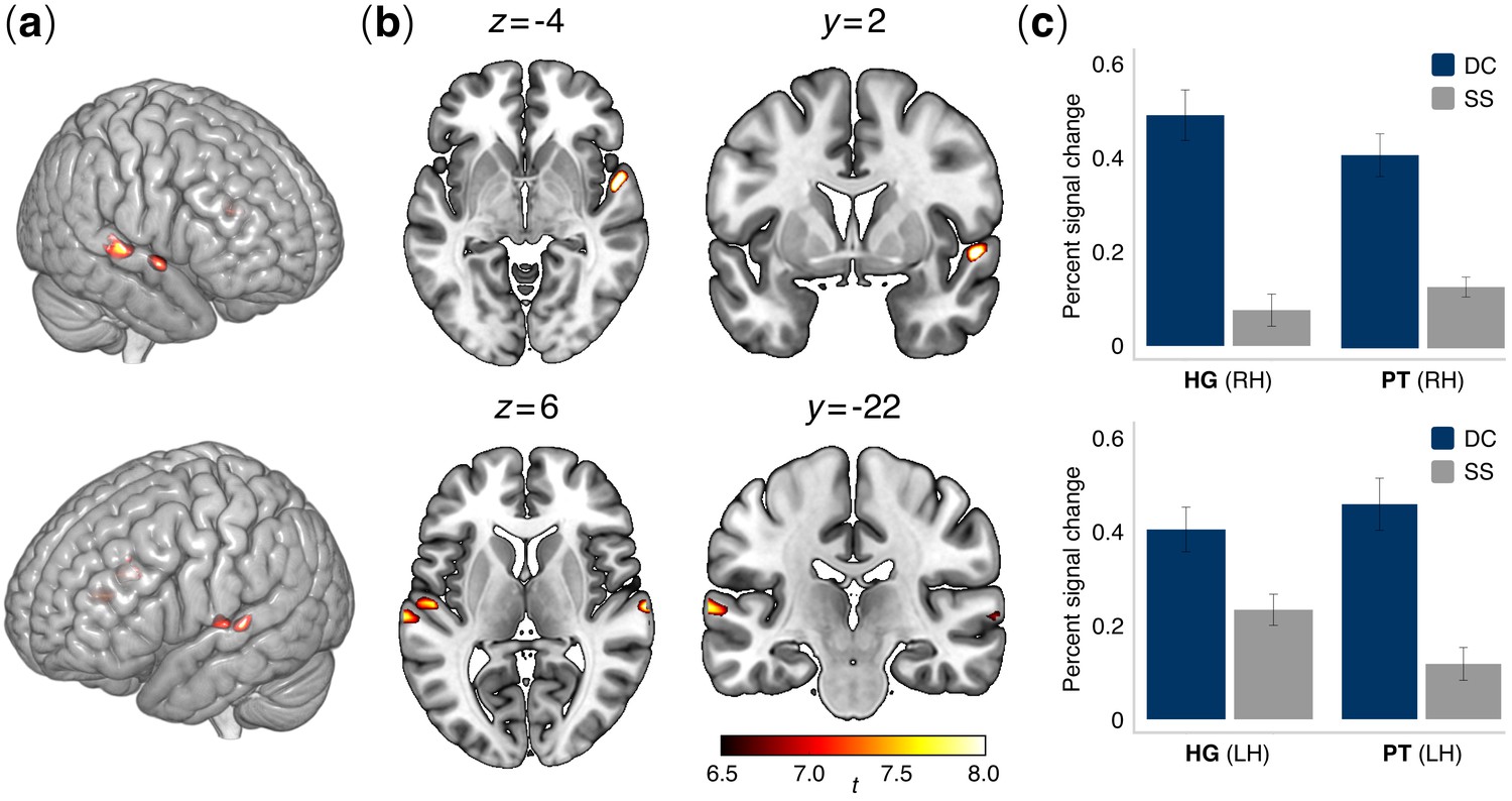
Brain activation patterns in the auditory functional localizer task.
(a) Lateral and (b) axial and coronal views of active voxels in temporal cortex overlaid onto an MNI standard brain for the contrast between contour deviant and standard stimuli (DC > SS). Significant activations were observed in the bilateral posterior superior temporal cortex, specifically in Heschl’s gyrus (HG) and the planum temporale (PT) bilaterally (see Table 2) (N = 52 participants). Contrasts were family-wise error (FWE) corrected for multiple comparisons at α = 0.001. Colormap intensities indicate indicate t-values. (c) Bar plots show percent changes in BOLD signal in HG and PT of the right hemisphere (upper panel) and left hemisphere (lower panel) in the comparison between contour deviants (DC) and standard sequences (SS). Error bars indicate the standard error of the mean.
Figure 5 with 1 supplement
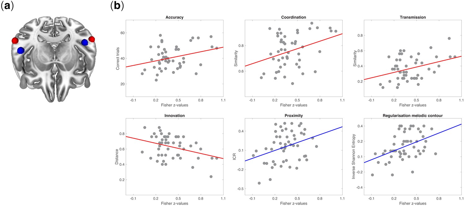
Neurobehavioral correlations.
(a) Tilted axial view of regions activated by the auditory functional localizer task in the posterior STG (red spheres) and anterior STG (blue spheres). (b) Pearson’s product-moment correlations between rs-FC (among regions activated in the functional localizer) and measures of behavior in signaling games: coordination (r = 0.41; p=0.002), accuracy (r = 0.36; p=0.007), transmission (r = 0.41; p=0.002), innovation (r = −0.41; p=0.003), proximity (r = 0.35; p=0.01), and regularization of melodic contour (r = 0.43; p=0.001). All p-values were Bonferroni corrected at α = 0.05/7 = 0.007. Fisher’s z-transformed correlation coefficients were obtained between pairs of 5 mm ROIs from session one and measures of behavior (accuracy, coordination, transmission, innovation) or structural features of tone sequences (proximity, regularization of melodic contours) from the signaling games on session 2. Behavioral measures were defined as the extent to which the code learned by a participant in Game 1 (accuracy and coordination) was faithfully recalled and transmitted in Game 2 (transmission) and reorganized between Games 1–2 (innovation). Each point on a scatterplot is one participant (N = 51).
Figure 5—figure supplement 1

Cross-correlation matrix showing.
Pearson’s correlation coefficients (Bonferroni-corrected for multiple comparisons at α = 0.05/10 = 0.005; 10 is the number of tests involving each variable). Abbreviations and variables are listed underneath the matrix.* p<0.005 CT: coordination tone; CC: coordination contour; IT: innovation tone; IC: innovation contour; TT: Transmission tone; TC: transmission contour; P: proximity; RT: regularization tone; RC: regularization contour; A: accuracy.
Figure 6
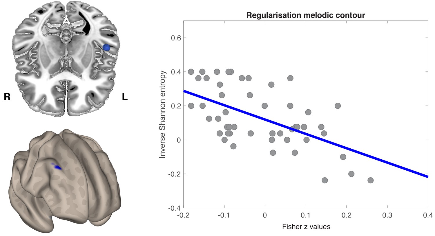
Seed-to-voxel regression analysis was conducted over the whole brain.
(a) Axial view of the left anterior STG (blue sphere) (top) and the voxel-wise FC correlation map (Fisher Z-transformed) (bottom). One cluster was identified by non-parametric permutation tests as showing a significant negative correlation between temporo-frontal connectivity values and melodic regularization (p<0.05, cluster-mass FWE corrected). (b) Pearson’s product moment correlation (r) between melodic regularization and mean FC connectivity between seed and all significant voxels in the frontal cluster (r = −0.58; p<0.001). Each point on a scatterplot is one participant (N = 51).
Tables
Table 1
Pearson product-moment correlations (r) between neural predictors (Fisher’s z-transformed ROI-to-ROI rs-FC values), neuropsychological predictors (digit span), and behavioral measures related to learning (coordination, transmission, innovation, accuracy) and structural regularization (proximity, melodic regularization).
https://doi.org/10.7554/eLife.48710.005| lHG- rHG | lHG- lSTG | lHG- rSTG | rHG- lSTG | rHG- rSTG | lSTG- rSTG | Digit Span | ||
|---|---|---|---|---|---|---|---|---|
| Learning | ||||||||
| Coordination | Tone | 0.05 | 0.26 | 0.10 | 0.17 | 0.12 | 0.41 | 0.22 |
| Contour | 0.15 | 0.33 | 0.13 | 0.10 | 0.02 | 0.35 | 0.11 | |
| Transmission | Tone | -0.09 | 0.23 | 0.01 | 0.13 | 0.14 | 0.41 | 0.11 |
| Contour | -0.08 | -0.04 | -0.05 | -0.10 | -0.04 | 0.009 | 0.008 | |
| Innovation | Tone | -0.01 | -0.41 | -0.10 | -0.20 | -0.12 | -0.40 | 0.05 |
| Contour | -0.03 | -0.10 | -0.05 | 0.01 | 0.004 | -0.04 | 0.08 | |
| Accuracy | -0.08 | 0.21 | 0.04 | 0.12 | -0.01 | 0.36 | 0.17 | |
| Structural regularization | ||||||||
| Proximity | 0.33 | 0.07 | 0.01 | 0.21 | 0.04 | -0.05 | -0.17 | |
| Melodic Regularization | Tone | 0.20 | -0.07 | -0.05 | 0.03 | -0.09 | -0.12 | -0.14 |
| Contour | 0.43 | 0.08 | 0.21 | 0.29 | 0.12 | 0.02 | -0.16 | |
-
Notes: Correlation coefficients marked in bold are significant under Bonferroni correction (α=0.05/7 = 0.007; seven is the number of independent tests on each behavioral variable). r = right hemisphere; l = left hemisphere. STG = superior temporal gyrus; HG = Heschl’s gyrus; Tone = measure computed using tone distance; Contour = measure computed using contour distance.
Table 2
Brain regions activated in the C-deviant >STD contrast (Height threshold: T = 6.76, pFWE <0.001; Extent threshold: k = 0 voxels).
https://doi.org/10.7554/eLife.48710.007| T statistic | MNI peak activation coordinates | Number of active voxels in the cluster | Anatomical region | Probabilistic atlas1 |
|---|---|---|---|---|
| 8.83 | [54 2 -4] | 54 | rSTG | Area TE (1.2) 28% OP4 (PV) 17% |
| 8.54 | [66 -16 4] | 60 | rSTG | Area TE (3) 57% |
| 7.93 | [−52–14 4] | 26 | lSTG | Area TE (1) 46% Area TE (1.2) 13% |
| 7.88 | [−66–22 6] | 32 | lSTG | Area TE (3) 73% |
-
Notes: Negative coordinates denote left-hemispheric regions. C-deviant = contour deviant; STD = standard; r = right hemisphere; l = left hemisphere. STG = superior temporal gyrus. FWE = familywise error corrected. 1Anatomical classification using the SPM anatomy toolbox (Eickhoff et al., 2005).
Additional files
-
Transparent reporting form
- https://doi.org/10.7554/eLife.48710.011
Download links
A two-part list of links to download the article, or parts of the article, in various formats.
Downloads (link to download the article as PDF)
Open citations (links to open the citations from this article in various online reference manager services)
Cite this article (links to download the citations from this article in formats compatible with various reference manager tools)
Functional connectivity in human auditory networks and the origins of variation in the transmission of musical systems
eLife 8:e48710.
https://doi.org/10.7554/eLife.48710


