Experimental investigation of ant traffic under crowded conditions
Figures
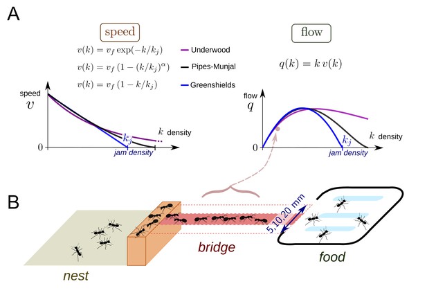
Theoretical fundamental diagrams and data collection.
(A) Three functions are often used to describe vehicular, fluid or pedestrian flows. The Greenshields function (Greenshields et al., 1935) was the first speed-density relation function used to analyze data recorded for vehicular traffic in the field. This function assumes a linear relationship between v and k leading to a parabolic shape relation between q and k. There are two parameters to be determined: the free speed vf corresponding to the speed of an individual without contact and the jam density kj, which is a threshold over which q becomes null. In the Pipes-Munjal function (Pipes, 1953), used for both pedestrians and car traffic, the relationship v - k is given by a power-law. This function requires a third parameter α to describe the function. The third function is the Underwood function (Underwood, 1960), which often describes well pedestrians or fluids traffic, where v decays exponentially rather than linearly. These functions made no a priori assumptions as to the behavior of the individuals and speed-density relationships are only obtained by fitting function to observed traffic data. (B) Experimental set-up. During an experiment, an ant colony (400 to 25,600 workers, 35 colonies in total) had access to a source of food (1M sucrose solution) placed at the end of a bridge (width: 5, 10 or 20 mm). The colonies were starved for five days before each experiment. The sucrose solution was spread over a large surface so that all ants had access to the food. The traffic on the bridge was recorded by a video camera for one hour. Inbound and outbound ants were counted over 1·sec intervals. Counting began as soon as the first ant crossed the middle of the bridge. A total of 170 experiments were performed.
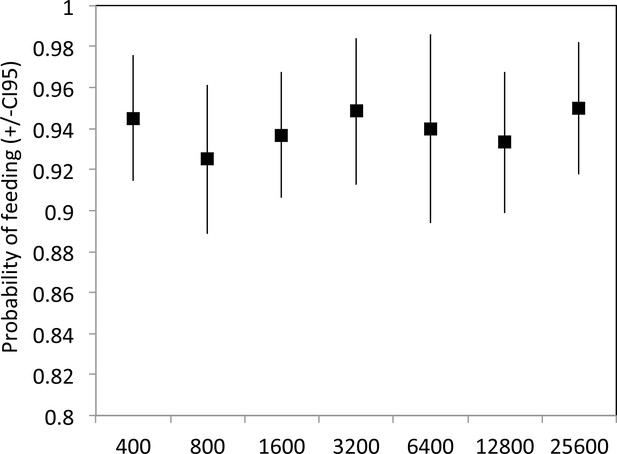
Probability of feeding when an ant reached the food as a function of colony size.
In average 94% of the ants fed once at the food source. N = 4200 ants followed across 42 experiments, two experiments for each experimental colony size and each bridge width (glmm, replicate and colony as a random factors, model for binomial data with logit function, Bridge width effect F = 0.67 p=0.521, Colony size effect F = 0.20 p=0.972, Bridge width*colony size F = 0.60 p=0.816). Error bars are CI95.
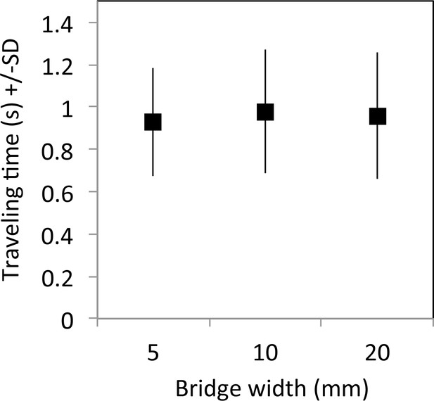
Travel time without contacts as a function of bridge width.
N = 2133 ants traveling a 2 cm section in the middle of the bridge in both directions; N = 34 experiments; one or two experiments for each experimental colony size and each bridge width. (glmm, replicate and colony as a random factors, Bridge effect F = 0.10 p=0.757, Colony size effect F = 2.88 p=0.090, Direction effect F = 2.83 p=0.092, all interactions were non significant). Error bars are SD.
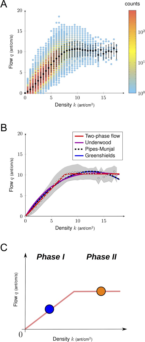
Empirical fundamental diagram.
(A) Density flow relationship. Both the density and the flow were measured over a time interval of one second and each point in the diagram corresponds to one data point (N = 612000 in total, N = 10303 for k > 8). Black dots indicate the mean and bars are standard deviations. (B) Non-linear fitting of the fundamental diagrams for the four functions tested (see Supplementary file 1). White dots represent the experimental mean flow and the gray region its standard deviation. (C) Illustration of a two phase flow diagram. At low density, the flow increases linearly with the density, whereas at large density the flow saturates and remains constant. Phase 1 (k < 8): q increases linearly with k, ants move freely. Phase 2 (k > 8): q stops increasing with k, but does not decay.
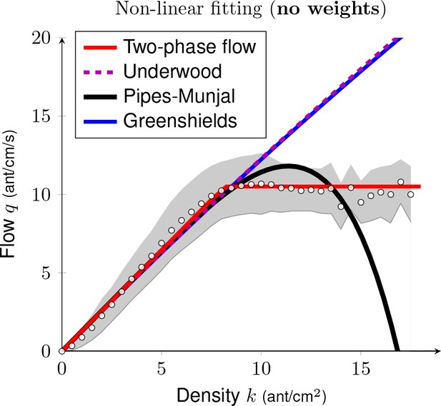
Non-linear fitting of the fundamental diagrams without weights.
Unlike the Figure 2B, no weights have been used to estimate the parameters of the four functions (see table S2). Only the two-phase flow function was able to capture the behavior for large density k when the flow reached a plateau for k > 8 ant.cm-2. White dots represent the experimental mean flow and the gray region its standard deviation.
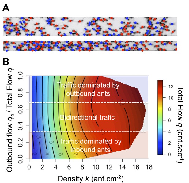
Spatial organization and flow asymmetry.
(A) Illustration of the ants’ spatial distribution on the 10 mm and 5 mm bridge. Colored dots correspond to travel direction. (B) Flow q (color scale) as a function of density k (x-axis) and asymmetry in the flows (y-axis). Traffic asymmetry was computed as the number of ants going to the food source per second (outbound flow) divided by the total number of ants traveling on the bridge (total flow q). When the proportion of outbound flow is 1 or 0 the traffic is unidirectional that is asymmetric, while if it is close to 0.5 the traffic is bidirectional that is symmetric. Red indicates the highest values for q on the response surface, with values descending to lowest values in dark blue regions. Response surfaces were visualized using non-parametric thin-plate splines, which were fitted using the fields package (Furrer et al., 2009) in the statistical software R version 3.5.0. The response surface regression analyses yielded significant relationships as follows: R2 = 0.82, p<0.001. The density is the main parameter affecting the flow while traffic asymmetry has only a marginal effect. Main effects: standardized beta βdensity = 0.980, βdensity2 = –0.126; Marginal effects: βAsymmetry2 = –0.040, βAsymmetry = 0.026 and βDensity*Asymmetry = 0.02. Flow isoclines run parallel to the Y-axis indicating that the flow depends mainly on density and is independent of traffic asymmetry.
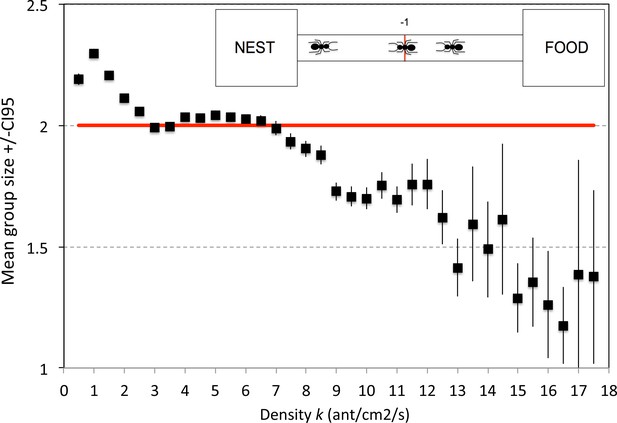
Temporal organization of the traffic.
For all experiments, we noted the travel direction for all successive ants crossing a line drawn on the middle (+1 for inbound ants, −1 for outbound ants). A group is defined as a succession of ant belonging to the same category (+1 or –1) and is delimited at both ends by ant belonging to the other category. The mean group size gives an indication of whether or not the sequence is random or if we can observe the formation of alternating groups of ants traveling in opposite direction. The mean group size (=2) obtained with a random sequence of ants generated on the basis of an equal probability of occurrence of nestbound and outbound ants is also represented as red line. Mean group sizes greater than two suggests the formation of alternating groups of inbound and outbound ants (sequence +1+1+1 −1-1-1 +1+1+1+1…) that is a temporal desynchronization of inbound and outbound traffic. Mean group size <<2 indicates that the outbound flow and the inbound flow are entirely intermingled (sequence +1–1+1–1+1–1+1–1+1…). N = 621,613 groups from 170 Experiments in total. Error bars are CI95.
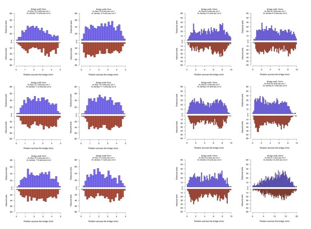
Spatial organization of the traffic.
For a subset of experiments (N = 12) characterized by a high traffic, we noted the travel direction for all ants crossing a line drawn on the middle (+one for inbound ants, −1 for outbound ants) and their y-position on this line for 240 consecutive seconds (using ImageJ). The measurements began 10·min after the beginning of the experiment, when the outbound and nestbound flows of ants were at equilibrium.

Flow q (y-axis) as a function of the asymmetry in the flows (x-axis) for three range of density k.
Traffic asymmetry was computed as the number of ants going to the food source per second (outbound flow) divided by the total number of ants traveling on the bridge (total flow q). When the proportion of outbound flow is 1 or 0 the traffic is unidirectional that is asymmetric while if it is close to 0.5 the traffic is bidirectional that is symmetric. Error bars are standard deviation and black dot represent the mean flow.
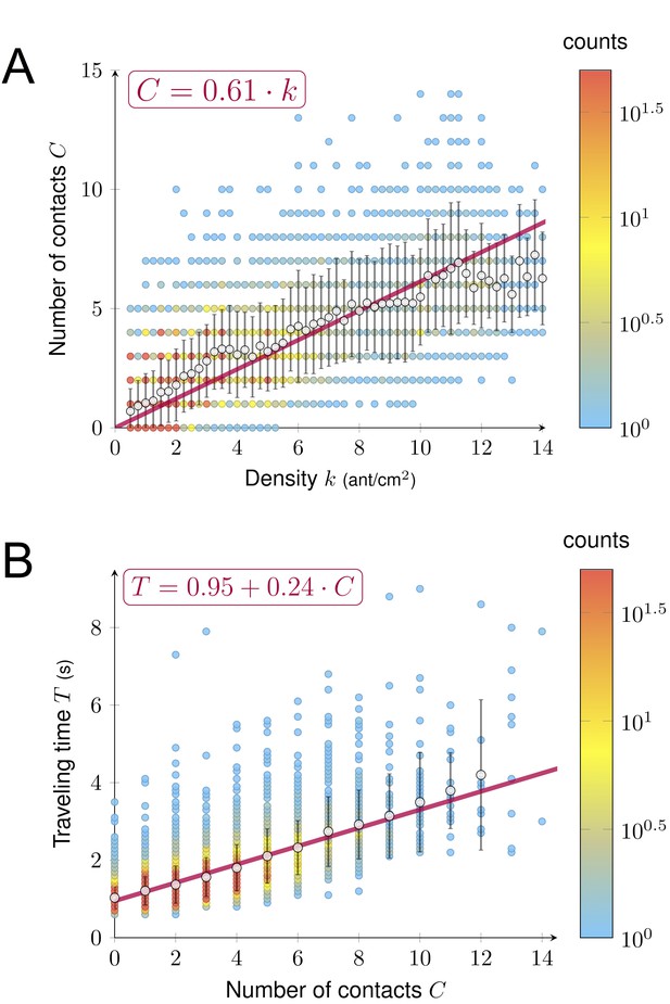
Relations between density, contact and traveling time.
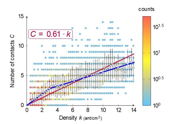
(A) Number of contacts C an ant incurred during the crossing of the bridge depending on the density k. C increased linearly with k (C = 0.61·k, R2 = 0.77). (B) Individual traveling time T as a function of the number of contacts C. T increased linearly with C (T = T0 + C · ∆T with free traveling time T0 = 0.95 s and time incurred by contact ∆T = 0.24 s, R2 = 0.55). We measured C along with k and the traveling time T for a sample of 7900 ants individually tracked on a 2 cm section at the center of the bridge (98 to 364 ants followed for each direction, each experimental group size and each bridge width). Data were collected 10·min after the beginning of the experiment, when the outbound and nestbound flows of ants were at equilibrium. Data were issued from 42 experiments in total. White dots represent average. Error bars are standard deviations.
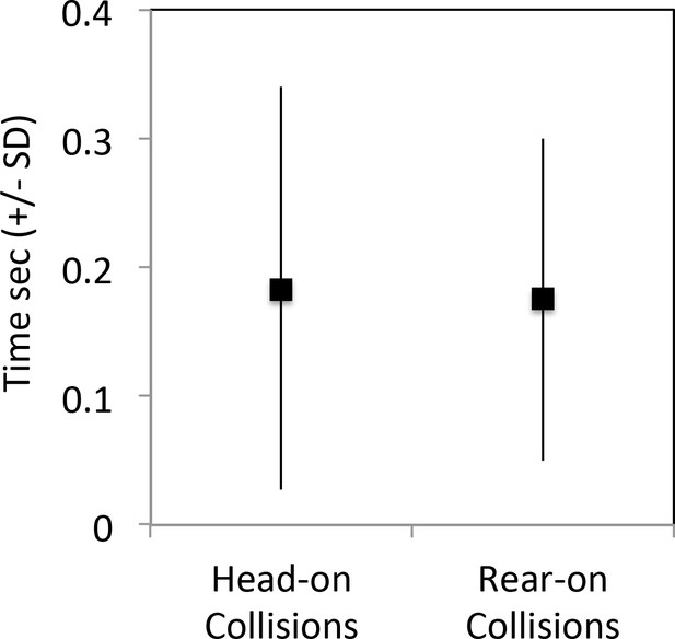
Time lost per contact as a function of collisions type.
Collisions obtained from the tracking of 5724 ants traveling a 2 cm section in the middle of the bridge in both directions. Data were issued from 38 experiments; one or two experiments for each experimental colony size and each bridge width. (glmm p=0.61, X2 = 0.25, random factors: experiment and individual).
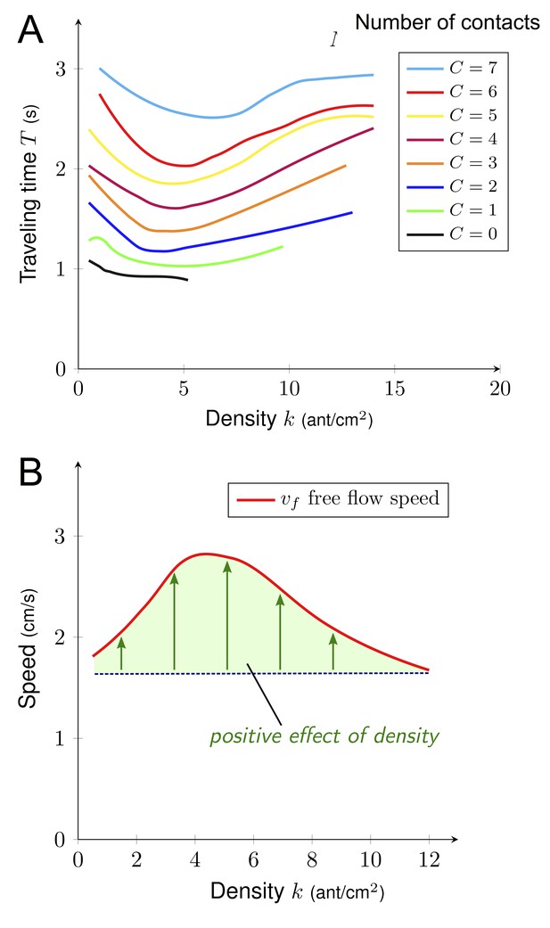
Free flow speed.
(A) Traveling time T depending on the density k for a given number of contacts C. Higher C induced longer T and T decreased until k reached 6. (B) Free flow velocity vf as a function of density. Free flow velocity is computed as the distance (L) divided by free traveling time T0 (traveling time without contact) that is vf = L/(T0) where L (2 cm) is the length of the monitoring section on the bridge. Hence, vf = L/(T-C·ΔT) as T0 = T C · ∆T (Figure 4B) where T is the individual traveling time, C is the number of contacts and ΔT (0.24 s) is the time incurred by contact. Data were collected for a sample of 7900 ants individually tracked on a 2 cm section (L) at the center of the bridge (98 to 364 ants followed for each direction, each experimental group size and each bridge width). Data were collected 10 min after the beginning of the experiment, when the outbound and nestbound flows of ants were at equilibrium. Data were issued from 42 experiments in total. Each curve was obtained by local regression fitting with R command loess.
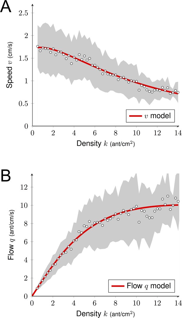
Predicted flow.
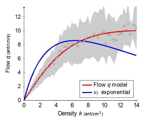
(A) Estimation of the speed v as a function of the density k. We combined positive and negative effects of the density k on v using Equation (2). Parameter estimation was done using non-linear regression method (R command nls). (B) Predicted flow q as a function of the density k using Figure 4 and Equation (3). We observed a linear growth of q (for k < 5–6), followed by a plateau (for k > 8). Experimental data correspond to the observations of a sub-sample dataset (7900 observations) from the full data set (612000 observations; Figure 2A) used to quantify the individual behavior. The gray shaded region represents the standard deviations. White dots are average computed from experimental data (N = 7,900). Data were collected 10 min after the beginning of the experiment, when the outbound and nestbound flows of ants were at equilibrium.
Videos
Ants traveling on a 20 mm wide bridge.
The video shows ants traveling between their nest and a food source 10·min after the beginning of the experiment, when the outbound and nestbound flows of ants were at equilibrium.
Ants traveling on a 5 mm wide bridge.
The video shows ants traveling between their nest and a food source 10·min after the beginning of the experiment, when the outbound and nestbound flows of ants were at equilibrium.
Additional files
-
Supplementary file 1
-Parameter estimations for the four functions.
(Table S1) Parameter estimations for the four functions with weight: To compensate for the discrepancy in the distribution of data points, we adjust the non-linear fitting by giving more weights for points under-represented (i.e.. increase weight ωi for large ki). More precisely, we compute the number Ni of data points for a given density value ki: Ni = #{(kn,qn) with kn = ki}. The weight is then given by ωii1/Ni. Using these weights corresponds to performing a fitting {ki, qi} with qi the average flow at k = ki. Parameter estimation with uniform weight is performed in Table S2. AW: Akaike weights, RSE: relative standard error. (Table S2) Parameter estimations for the four functions without weight. Unlike the Table S1, the parameter estimations use a non-linear regression using all points with the same weight ω = 1.
- https://doi.org/10.7554/eLife.48945.018
-
Transparent reporting form
- https://doi.org/10.7554/eLife.48945.019


