Figures and data in Multistability and regime shifts in microbial communities explained by competition for essential nutrients | eLife

Figures
Additional files

6 figures and 7 additional files

Figures

Figure 1 with 1 supplement

Download asset Open asset

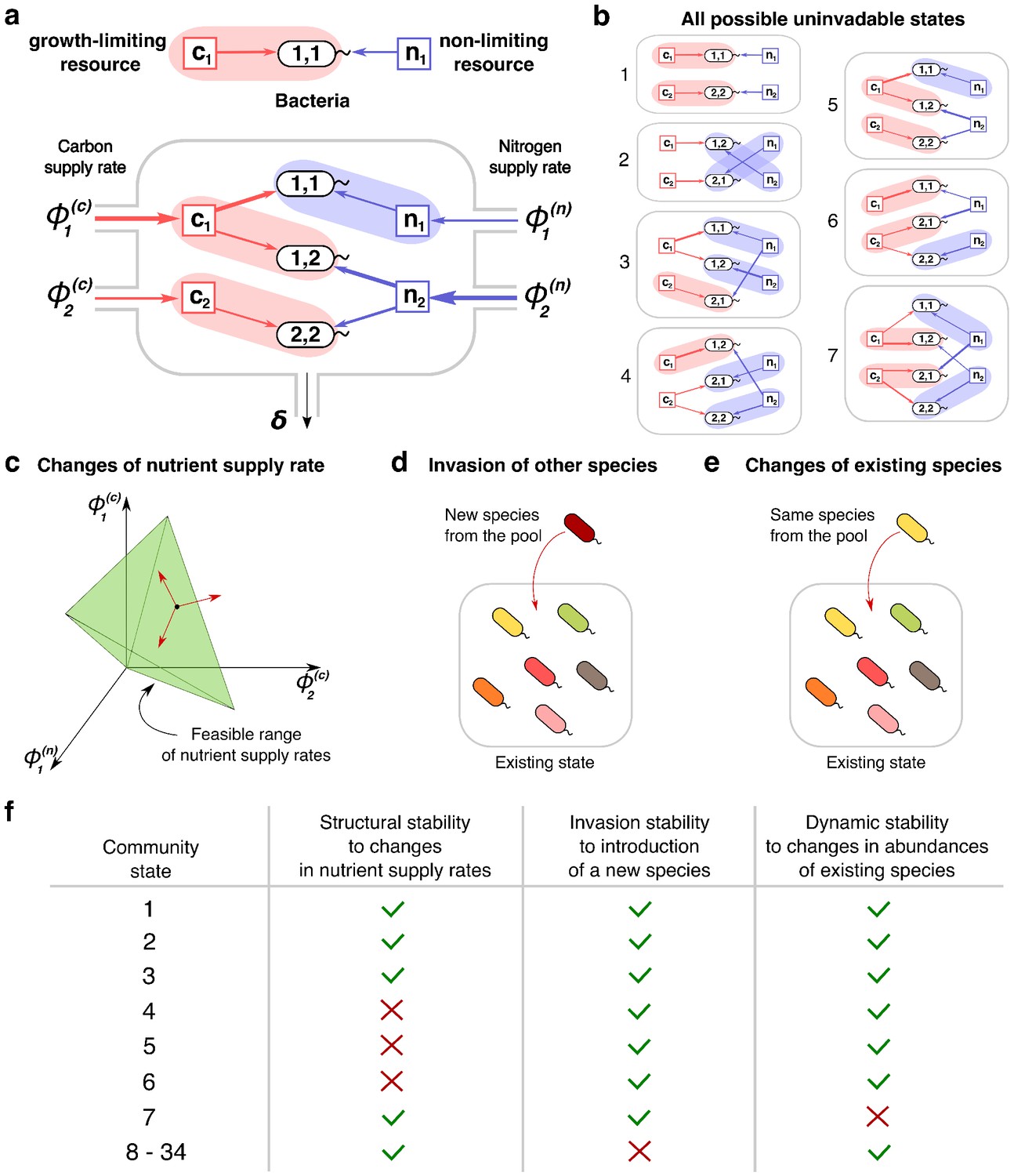
Community states and different types of their stability.

(a) A schematic depiction of the proposed experimental setup and one of several possible community states in the 2C × 2N × 4S model. Several sources of carbon an nitrogen are supplied at constant rates $ϕ_{i}^{(c)}$ and $ϕ_{j}^{(n)}$ to a chemostat with a dilution rate $δ$ . Red and blue square nodes represent these nutrients inside the chemostat with steady state concentrations $c_{1}$ , $c_{2}$ (for carbon) and $n_{1}$ , $n_{2}$ (for nitrogen). They are consumed by three microbial species labeled by the pair of carbon (the first index) and nitrogen (the second index) nutrients this species consumes. Shaded ovals connect every species to its unique growth-limiting nutrient. The fourth species $B_{2, 1}$ is not present in this steady state. (b) All seven uninvadable states in our realization of 2C × 2N × 4S model (see Supplementary files 1,2 for the specific parameters). depicted using the same schematic representation as in (a). Panels (c–e) schematically illustrate three possible types of perturbations of a community state, corresponding to three different types of its stability. (c) Changes of nutrient supply rates, that may result in extinction of some of the species. Green shaded area schematically depicts the region of nutrient supply rates where a given state is feasible, red arrows represent the perturbations of nutrient supply rates. (d) Introduction of species currently absent from the system, that is invasion, that may change the set of surviving species. (e) Small fluctuations in abundances of existing species, that may disturb the dynamic equilibrium of the system and potentially drive it to another state. (f) Table that shows which stability criteria are satisfied for 34 possible states in our realization of 2C × 2N × 4S model. Note that these types of stability are in general unrelated to each other.

Figure 1—figure supplement 1

Download asset Open asset

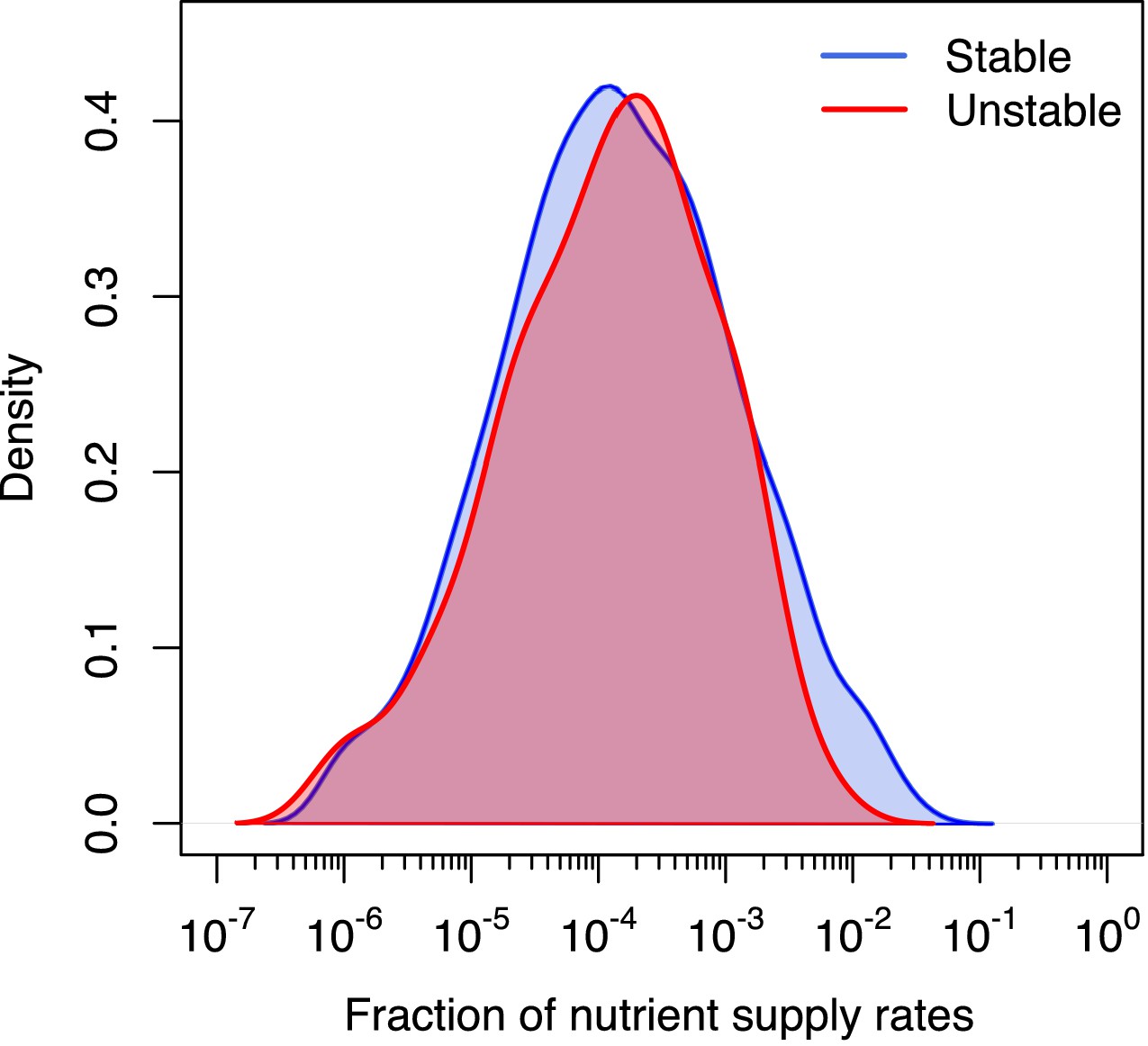
Distribution of volumes for stable and unstable states.

Log-normal distribution of feasible volumes of 1211 uninvadable states in 6C × 6N × 36S version of our model. Red line is used for 1058 dynamically stable states and blue line for 153 dynamically unstable ones. Distributions are normalized to the total number of states of each type. The natural logarithm of the volume has mean $μ = - 8.87 \pm 0.06$ and standard deviation $σ = 2.08 \pm 0.04$ . There is no significant difference between distributions of volumes of stable and unstable uninvadable states (two-sample Kolmogorov-Smirnov test: p-value = 0.94).

Figure 2 with 1 supplement

Download asset Open asset

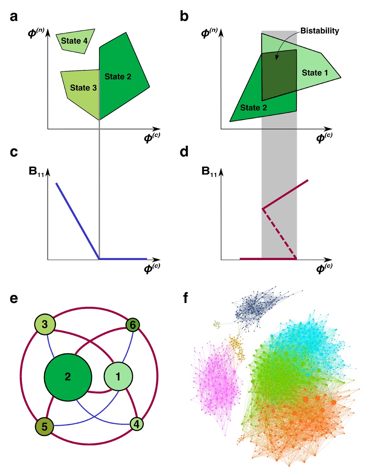
Regime shifts between alternative stable states.

(a) Shaded green areas schematically depict the feasible ranges of nutrient supply rates for several stable states in our model (#2-#4 in Figure 1B). The feasible range of the state #4 does not overlap with that of any other state. Feasible ranges of states #2 and #3 also do not overlap but share a common boundary. Panel (b) depicts the opposite scenario of overlapping feasible ranges of another pair of stable states (#1 and #2 in Figure 1B). In the overlapping region (dark green), they form a pair of alternative stable states. (c) A smooth transition between two states at the boundary. The population $B_{11}$ of the microbial species (1,1) is plotted as a function of changing nutrient supply rate $ϕ^{(c)}$ (same as the x-axis in panel (a)). Vertical gray line corresponds to the boundary between states #3 and #2. (d) A regime shift between two states. $B_{11}$ is plotted as a function of nutrient supply $ϕ^{(c)}$ as it sweeps through the overlapping region (gray area) in panel (b). Note abrupt changes of $B_{11}$ at the boundaries of the overlapping region and its hysteretic behavior as expected for regime shifts. Dashed line corresponds to $B_{11}$ in a dynamically unstable state (#7 in Figure 1B). (e) The network of possible regime shifts between pairs of stable states in the 2C × 2N × 4S model. Each red edge represents a possible regime shift between two states it connects (overlap of their feasible ranges as in panel (d)). Each blue edge corresponds to a smooth transition between two states while changing the fluxes (as in panel (c)). Nodes correspond to six uninvadable and dynamically stable states (state labels are the same as in Figure 1b). Sizes of nodes reflect relative magnitudes of feasible ranges of states they represent. (f) Network of 8633 possible regime shifts between pairs of 893 uninvadable dynamically stable states in the 6C × 6N × 36S model. The size of each node reflects its degree (i.e. the total number of other stable states that a given state can shift into). The color of each node corresponds to its network modularity class calculated as described in Materials and methods.

Figure 2—figure supplement 1

Download asset Open asset

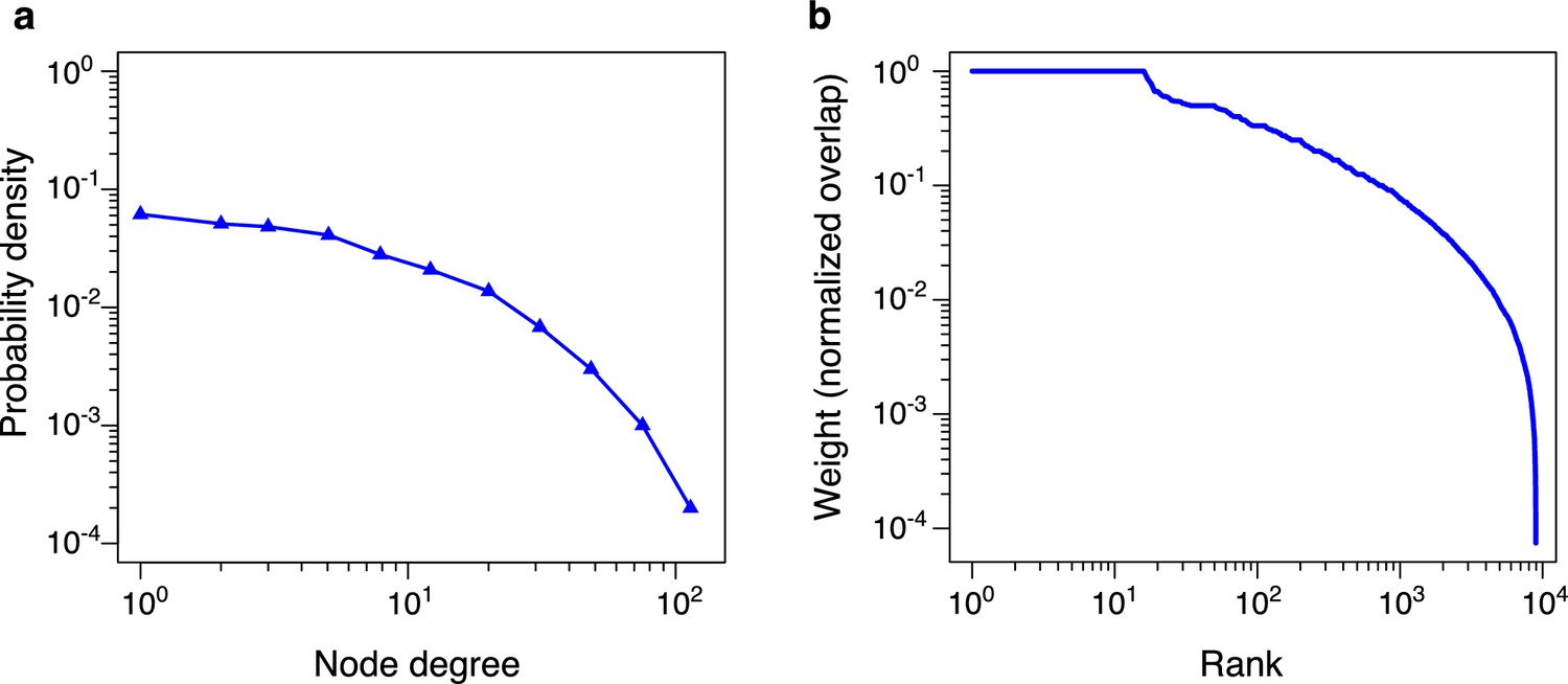
Statistics of pairwise bistability network for 6C × 6N × 36S example.

(a) Degree distribution of the network in Figure 2F. (b) Rank-ordered distribution of weights of network edges from Figure 2F. The weights of the network in Figure 2F are given by normalized overlaps between states.

Figure 3 with 1 supplement

Download asset Open asset

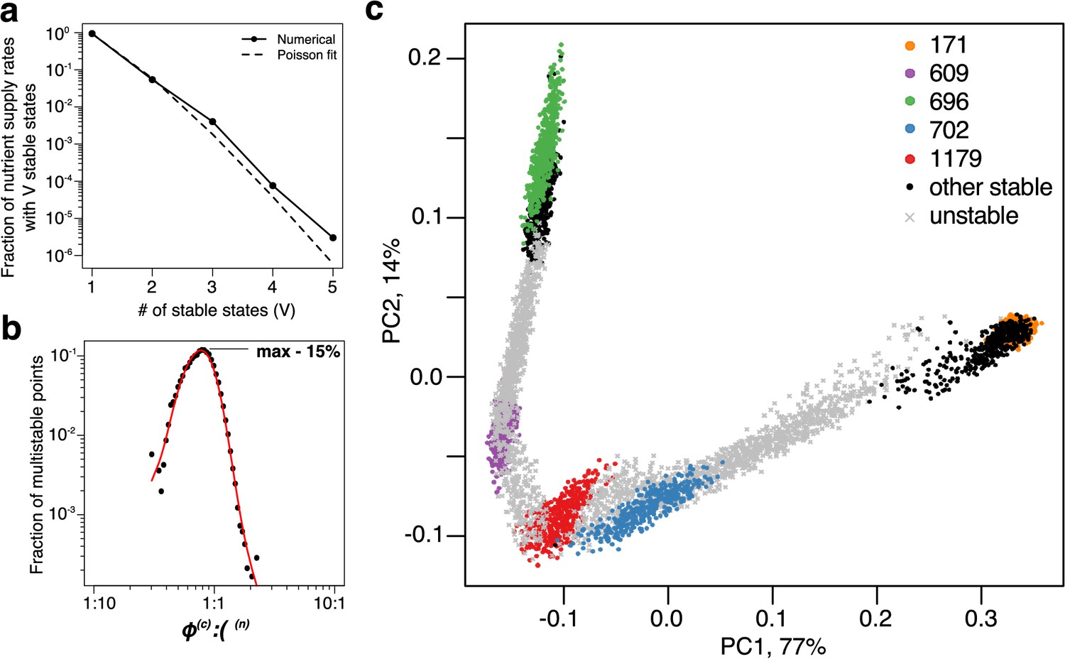
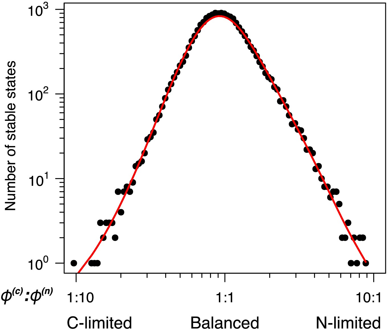
Patterns of multistability.

(a) The distribution of the number, $V$ , of multistable states across the entire space of nutrient supply rates. The data is based on Monte Carlo sampling of 1 million different environments (combinations of nutrient supply rates) in the 6C × 6N × 36S model. Solid circles show the fraction of all sampled environments for which $V = 1, 2, 3, 4, 5$ uninvadable dynamically stable states are simultaneously feasible. The dashed line is the fit to the data with a Poisson distribution for $v - 1$ extra states giving rise to multistability. (b) Fraction of multistable cases for different ratios of supply of two essential nutrients. The peak of the distribution is close to the balanced supply ( $ϕ^{(c)} : ϕ^{(n)} ≃ 1 : 1$ ). (c) The PCA plot of relative microbial abundances in the vicinity of the environment, where $V = 5$ stable states coexist. Supply rates were randomly sampled within ±10% from the initial environment. Each point shows the first (x-axis) and the second (y-axis) principal components of microbial abundances in every uninvadable state feasible for this combination of supply rates. Colored circles label the original five stable states, black circles - several other stable states, which became feasible for nearby supply rates, and grey crosses - dynamically unstable states feasible in this region of nutrient supply rates.

Figure 3—figure supplement 1

Download asset Open asset

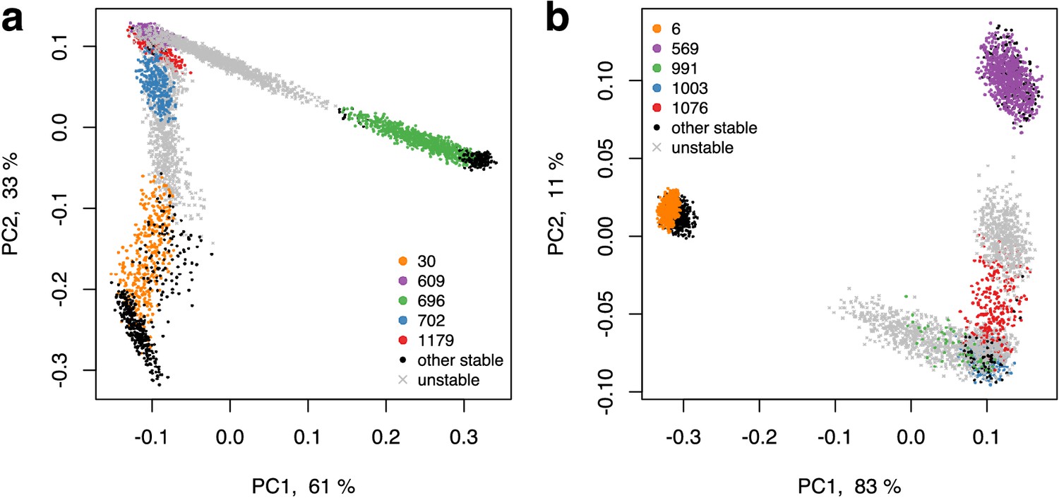
The PCA plot of fractional microbial abundances.

These abundances, normalized to 1, were obtained in our simulations for supply rates in the local vicinity of a multistable point where $V = 5$ stable states coexist. Panels (a) and (b) represent the two remaining multistable points in addition to the multistable point shown in Figure 3C. Axes show the percentage of the variance explained by each principal component. Each point show the first (x-axis) and the second (y-axis) principal coordinates of microbial abundances in an uninvadable state feasible for a given set of nutrient supply rates. The supply rates were chosen to be close (±10%) to the initial multistable point. Colored circles mark the original five stable states, black circles - other stable states which became feasible for nearby supply rates, and grey crosses - dynamically unstable states feasible in this influx region. Note a quasi-1D manifold along which the points of all colors are aligned and the alternating order of points corresponding to stable and unstable states.

Figure 4 with 1 supplement

Download asset Open asset

Patterns of diversity and structural stability of states.

(a) Average species richness (y-axis) of uninvadable stable states feasible for a given $ϕ^{(c)} : ϕ^{(n)}$ nutrient supply ratio (x-axis). Error bars correspond to standard deviation of species richness of individual states feasible for a given nutrient supply ratio (see Figure 4—figure supplement 1 for the number of states contributing to each point). (b): Scatter plot of the prevalence (y-axis) of each of the 36 species in the 6C × 6N × 36S model plotted vs its average competitiveness rank for its carbon and nitrogen sources. The latter is calculated from the rank order of $λ^{(c)}$ and $λ^{(n)}$ among all species consuming each resource (rank one corresponds to the largest $λ$ for this resource among all species). Species prevalence is quantified as the fraction of environments where a given species can survive. The dashed line shows the average trend. (c) The number of uninvadable dynamically stable (solid line) and unstable (dashed line) states with a particular species richness (x-axis). (d) Boxplot of nutrient feasibility ranges of uninvadable stable states plotted as a function of their species richness. All plots were calculated for the 6C × 6N × 36S model.

Figure 4—figure supplement 1

Download asset Open asset

Number of unique uninvadable stable states that are feasible for a given $ϕ^{(c)} : ϕ^{(n)}$ nutrient supply ratio (x-axis is binned as in Figure 4A).

Figure 5

Download asset Open asset

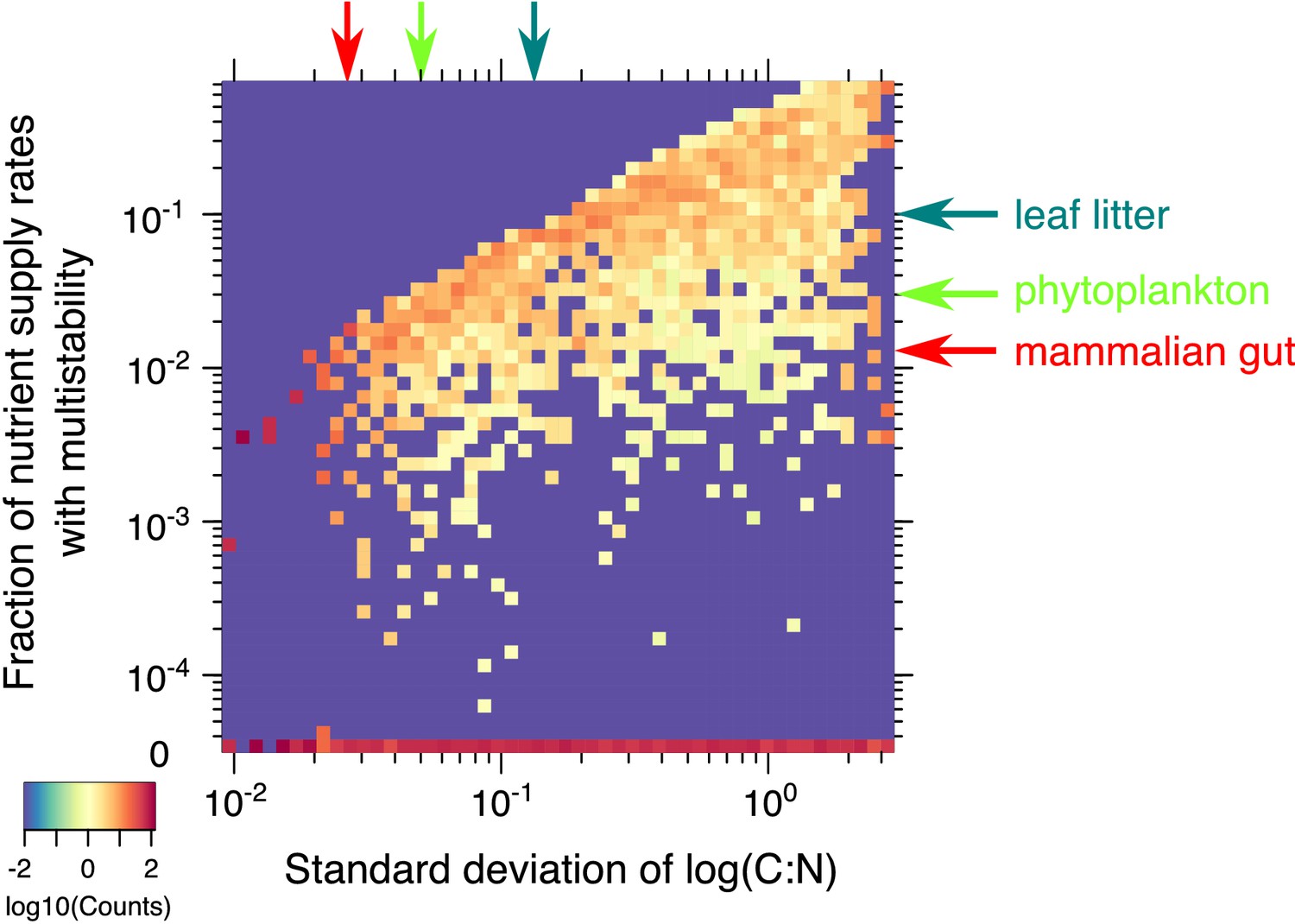
Statistics of multistability for different combinations of yields.

Heatmap of the fraction of nutrient supply rate combinations that permit multistability for the 2C × 2N × 4S model with the same set of $λ$ ’s but different combinations of microbial growth yields (4000 model variants in total). Standard deviations of yields (x-axis) and the fraction of nutrient supply rates with multistability (y-axis) were logarithmically binned into 50 bins along each axis. The color scale represents log10 of the normalized count in each bin. The counts were normalized to add up to 100% in each column (same bin of the x-axis) to approximate the probability distribution of multistability fraction for given standard deviation of species stoichiometry. The bottom row (0) corresponds to 2069 yields combinations where no multistability was observed for any nutrient supply combinations in our Monte-Carlo simulations of 10⁶ flux points. The red arrow on the x-axis corresponds to the approximate yield variation for mammalian gut microbes from Reese et al. (2018). The red arrow on y-axis highlights the predicted likelihood of multistability in our model for a microbial community with the same yield variation in our model. Light green arrows show an estimation of these numbers for phytoplankton species from Finkel et al. (2016). Dark green arrows correspond to the soil microbes studied in Mouginot et al. (2014).

Appendix 3—figure 1

Download asset Open asset

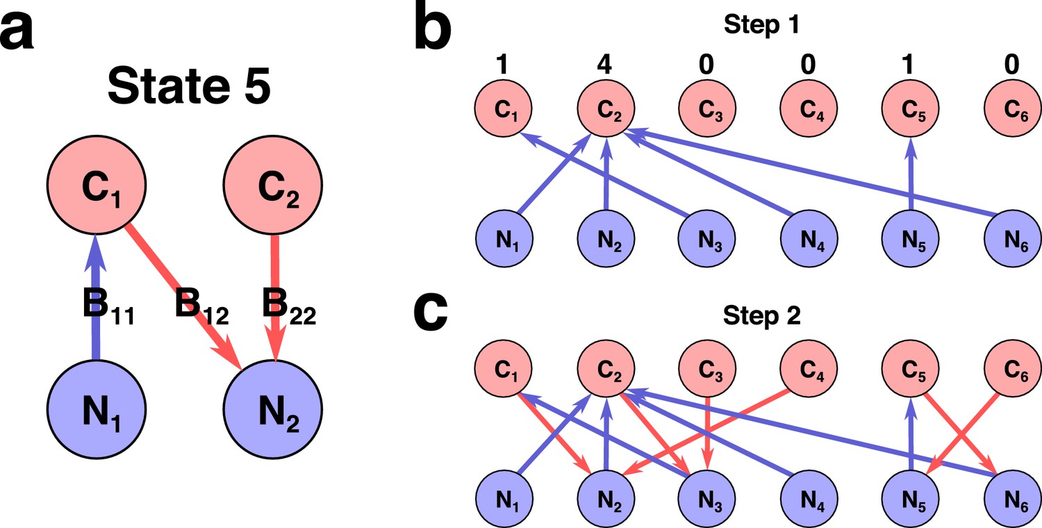
Network representation of a state in Stable Marriage analogy.

(a) Schematic representation of state #5 in the 2C × 2N × 4S model (the same state is shown in Figure 1A in Main text). Here each species represented as an arrow connecting two resources it is utilizing for growth, with the color and direction of arrow representing growth-limitation of a species (red corresponds to C-limited species, blue N-limited one). (b)-(c) Schematic representation of two-step construction of state #991 in the 6C × 6N × 36S model. (b) We first assign all species that are growth-limited by N (blue links outgoing from N sources). The numbers above C sources indicate number of vacancies for a given resource. (c) Then for a given set of N-limited species we populate the remaining C-limited ones that are allowed by the Condition 2 (red links outgoing from C sources).

Additional files

Supplementary file 1 Values of species’ competitive abilities for carbon and nitrogen in 2C × 2N × 4S model.: https://cdn.elifesciences.org/articles/49720/elife-49720-supp1-v1.xlsx
Download elife-49720-supp1-v1.xlsx
Supplementary file 2 Values of species’ carbon and nitrogen yields in 2C × 2N × 4S model.: https://cdn.elifesciences.org/articles/49720/elife-49720-supp2-v1.xlsx
Download elife-49720-supp2-v1.xlsx
Supplementary file 3 Values of species’ competitive abilities for carbon in 6C × 6N × 36S model.: https://cdn.elifesciences.org/articles/49720/elife-49720-supp3-v1.xlsx
Download elife-49720-supp3-v1.xlsx
Supplementary file 4 Values of species’ competitive abilities for nitrogen in 6C × 6N × 36S model.: https://cdn.elifesciences.org/articles/49720/elife-49720-supp4-v1.xlsx
Download elife-49720-supp4-v1.xlsx
Supplementary file 5 Values of species’ carbon yields in 6C × 6N × 36S model.: https://cdn.elifesciences.org/articles/49720/elife-49720-supp5-v1.xlsx
Download elife-49720-supp5-v1.xlsx
Supplementary file 6 Values of species’ nitrogen yields in 6C × 6N × 36S model.: https://cdn.elifesciences.org/articles/49720/elife-49720-supp6-v1.xlsx
Download elife-49720-supp6-v1.xlsx
Transparent reporting form: https://cdn.elifesciences.org/articles/49720/elife-49720-transrepform-v1.docx
Download elife-49720-transrepform-v1.docx

Download links

A two-part list of links to download the article, or parts of the article, in various formats.

Downloads (link to download the article as PDF)

Open citations (links to open the citations from this article in various online reference manager services)

Mendeley

Cite this article (links to download the citations from this article in formats compatible with various reference manager tools)

Veronika Dubinkina
Yulia Fridman
Parth Pratim Pandey
Sergei Maslov

(2019)

Multistability and regime shifts in microbial communities explained by competition for essential nutrients

eLife 8:e49720.

https://doi.org/10.7554/eLife.49720

Sign up for email alerts

Privacy notice