Stability and asynchrony of local communities but less so diversity increase regional stability of Inner Mongolian grassland
- Ministry of Education Key Laboratory of Ecology and Resource Use of the Mongolian Plateau & Inner Mongolia Key Laboratory of Grassland Ecology, School of Ecology and Environment, Inner Mongolia University, China
- Institute of Ecology, College of Urban and Environmental Sciences, and Key Laboratory for Earth Surface Processes of the Ministry of Education, Peking University, China
- Department of Geography, Remote Sensing Laboratories, University of Zürich, Switzerland
Figures
Box 1—figure 1
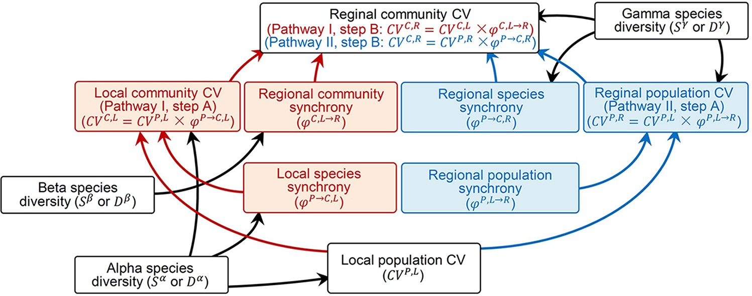
Upscaling local population coefficient of variation (CV) to regional community CV via local community CV (pathway I, red arrows on the left side) and regional population CV (pathway II, blue arrows on the right side), as well as theoretically proposed impacts of species diversity measures on them.
Figure 1 with 1 supplement
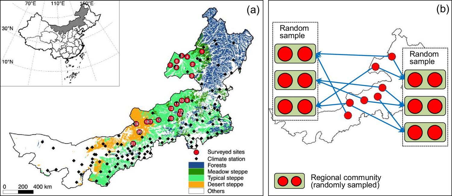
Geographic distribution of surveyed sites with site numbers (a) and a simplified case (seven-site) for illustrating construction of regional communities aggregating two local communities (b).
In (a), red circles represent sites included in constructing regional communities. (b) shows a simplified case illustrating the construction of two sets of regional communities using random sampling without replacement to ensure the regional communities within each set do not share local communities.
Figure 1—figure supplement 1
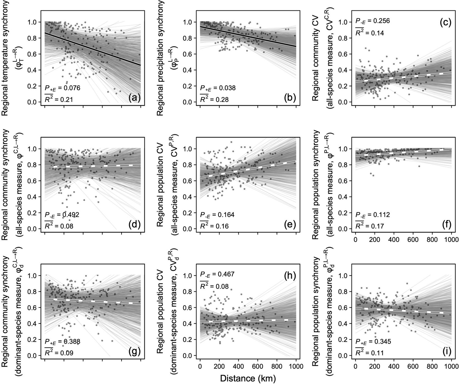
Regional synchronies of temperature (a) and precipitation (b), all-species measure of regional community coefficient of variation (CV, inverse of stability, c) and all-species (d–f) and dominant-species (g–i) measures of regional community synchrony (inverse of asynchrony), regional population CV, and regional population synchrony in relation to distance.
Solid black lines represent significant (p<0.05) and marginally significant (p<0.10) relationships, and dashed gray line represents nonsignificant (p>0.10) relationships (see ‘Materials and methods’ for details and Box 1 for glossary). Thin grey lines represent relationships for 1000 sets of resampled regional communities (n=10 for each set). Symbols and descriptions can be found in Box 1 and Appendix 1—table 1. Dataset and code are in available in Figshare at https://doi.org/10.6084/m9.figshare.20281902.
Figure 2 with 1 supplement

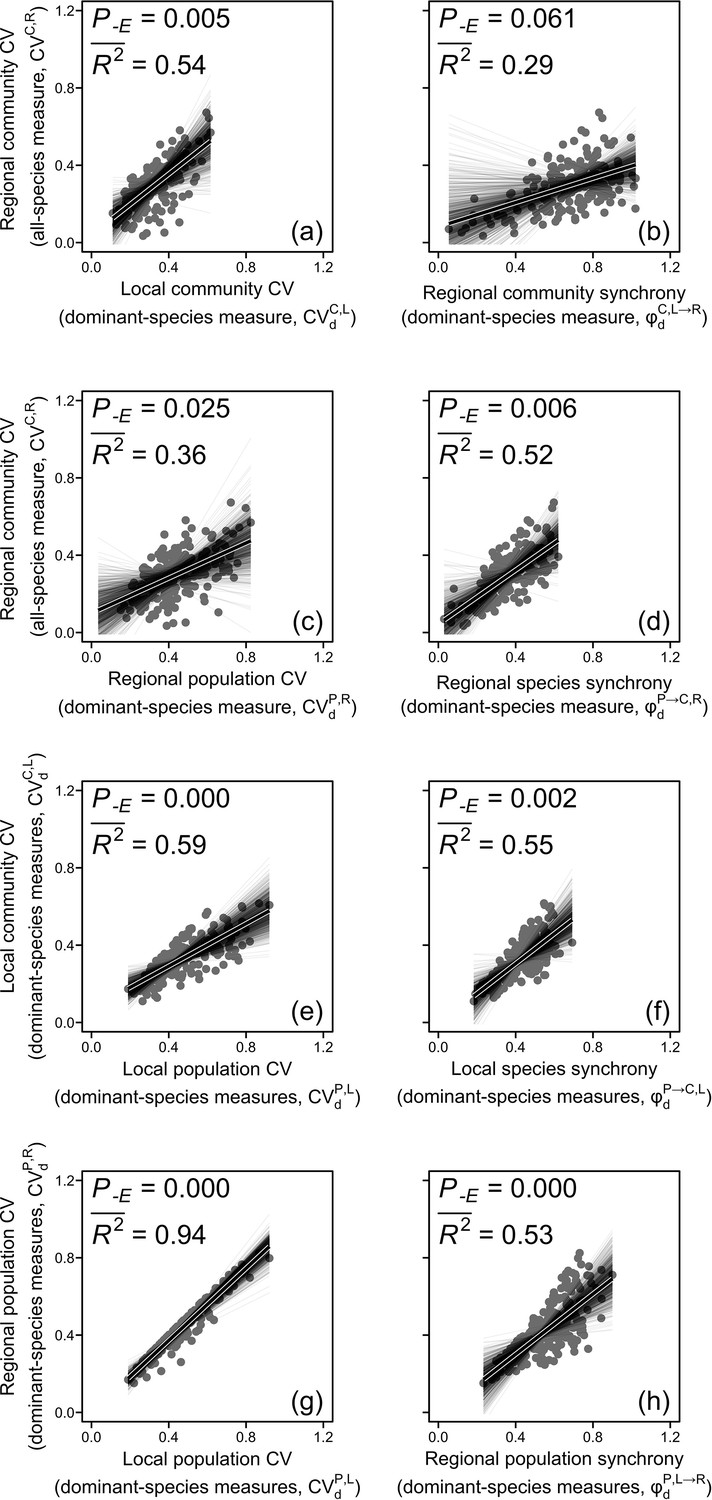
The regional community (a–d), local community (e–f), and regional population (g–h) coefficients of variation (CVs) in relation to their hierarchical components using all-species measures.
Solid black lines represent significant (p<0.05) and marginally significant (p<0.10) relationships, and dashed gray lines represent nonsignificant (p>0.10) relationships (see ‘Materials and methods’ for details and Box 1 for glossary). Thin grey lines represent relationships for 1000 sets of resampled regional communities (n=10 for each set). See Figure 2—figure supplement 1 for results of using dominant-species measures. Dataset and code are available in Figshare at https://doi.org/10.6084/m9.figshare.20281902.
Figure 2—figure supplement 1
All-species estimate of regional community coefficient of variation (CV, inverse of stability) in relation to dominant-species estimates of local community CV (a), regional community synchrony (inverse of asynchrony, b), regional population CV (c), and synchrony (d) as well as dominant-species estimates of local community CV (e, f) and regional population CV (g, h) in relation to their hierarchical components.
Solid black lines represent significant (p<0.05) and marginally significant (p<0.10) relationships, and dashed gray lines represent nonsignificant (p>0.10) relationships (see ‘Materials and methods’ for details and Box 1 for glossary). Thin grey lines represent relationships for 1000 sets of resampled regional communities (n=10 for each set). Dataset and code are available in Figshare at https://doi.org/10.6084/m9.figshare.20281902.
Figure 3 with 1 supplement
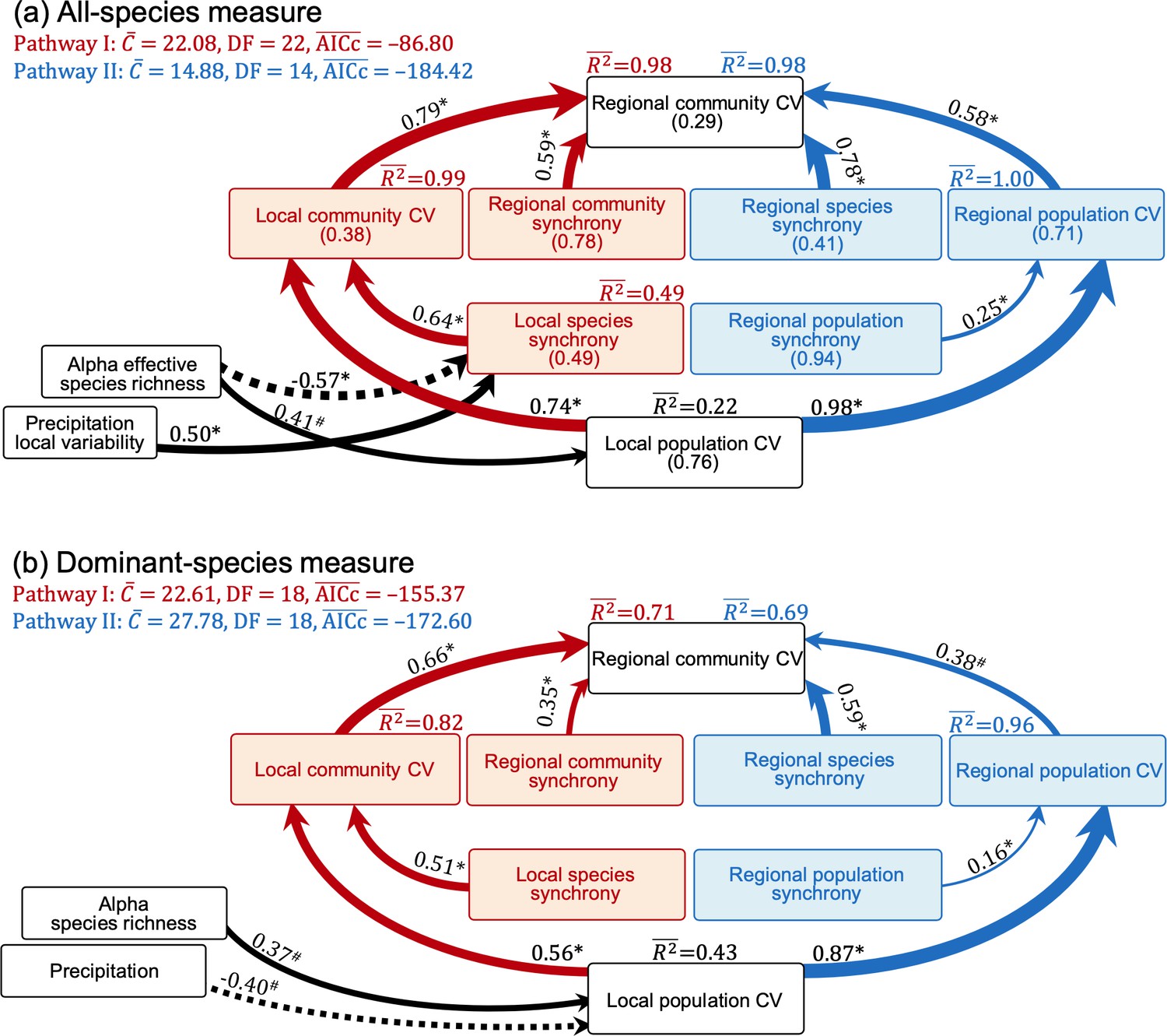
Path analysis models relating the regional community coefficient of variation (CV, all-species measure) to its hierarchical components and species diversity indices estimated with all species (a, the mean values of CVs and synchronies are in brackets) and only dominant species (b) as well as climatic factors.
These diagrams combine different upscaling pathways (pathway I, left side with red arrows; pathway II, right side with blue arrows). Solid and dashed arrows, respectively, represent positive and negative paths, and numbers near arrows are standardized path coefficients. The significance level of each path is indicated by * when p<0.05 or # when p<0.10 (see ‘Materials and methods’ for details and Box 1 for glossary). See Figure 3—figure supplement 1 for relationships between all-species and dominant-species measures. Dataset and code are available in Figshare at https://doi.org/10.6084/m9.figshare.20281902.
Figure 3—figure supplement 1
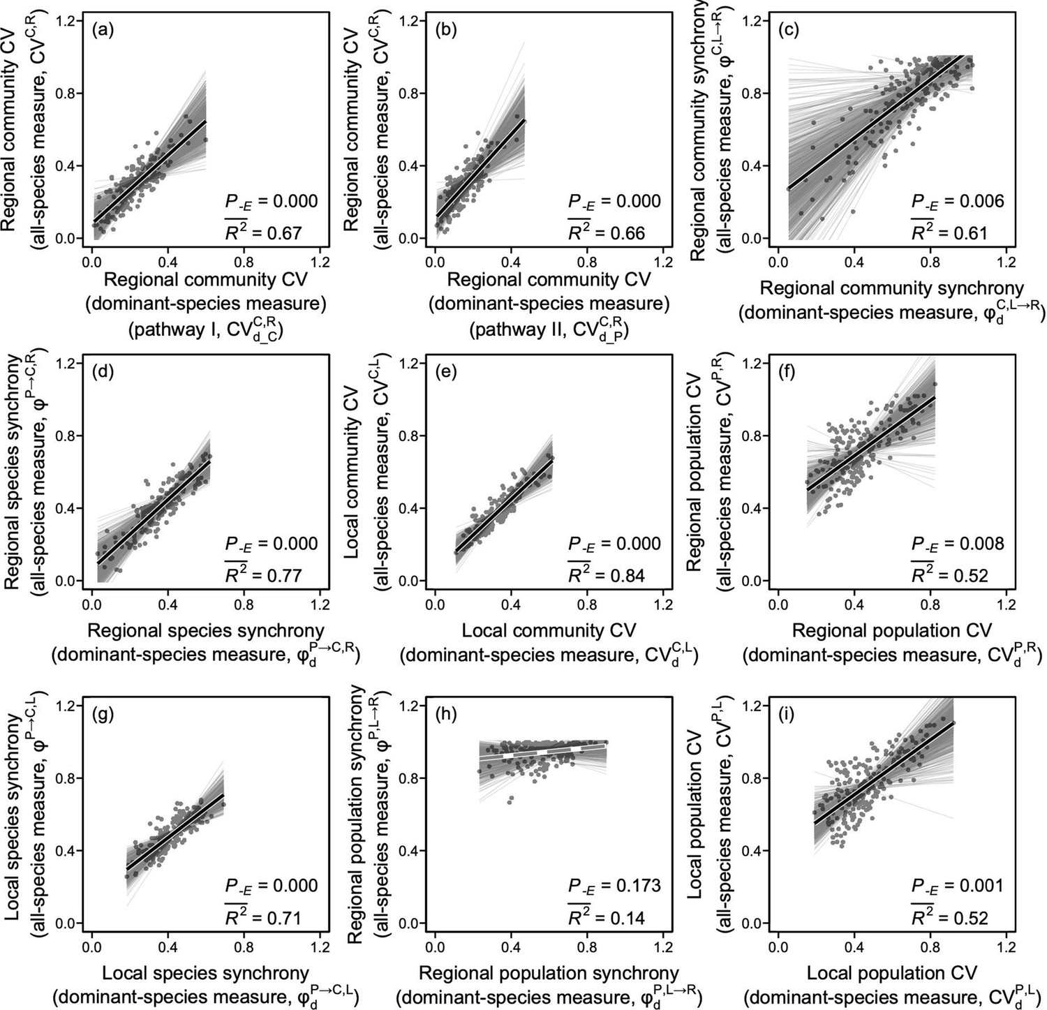
All-species estimates (vertical axes) of coefficients of variation (CVs, inverse of stability) and synchronies (inverse of asynchrony) across hierarchical levels of ecological organization in relation to their dominant-species counterparts (horizontal axes) (a–b, regional community CV; c, regional community synchrony; d, regional species synchrony; e, local community CV; f, regional population CV; g, local species synchrony; h, regional population synchrony; i, local population CV).
Solid black lines represent significant (p<0.05) and marginally significant (p<0.10) relationships, and dashed gray line represents nonsignificant (p>0.10) relationship (see ‘Materials and methods’ for details, Box 1 for glossary and Appendix 1–1.6 for dominant-species measures). Thin grey lines represent relationships for 1000 sets of resampled regional communities (n=10 for each set). Dataset and code are available in Figshare at https://doi.org/10.6084/m9.figshare.20281902.
Figure 4 with 1 supplement
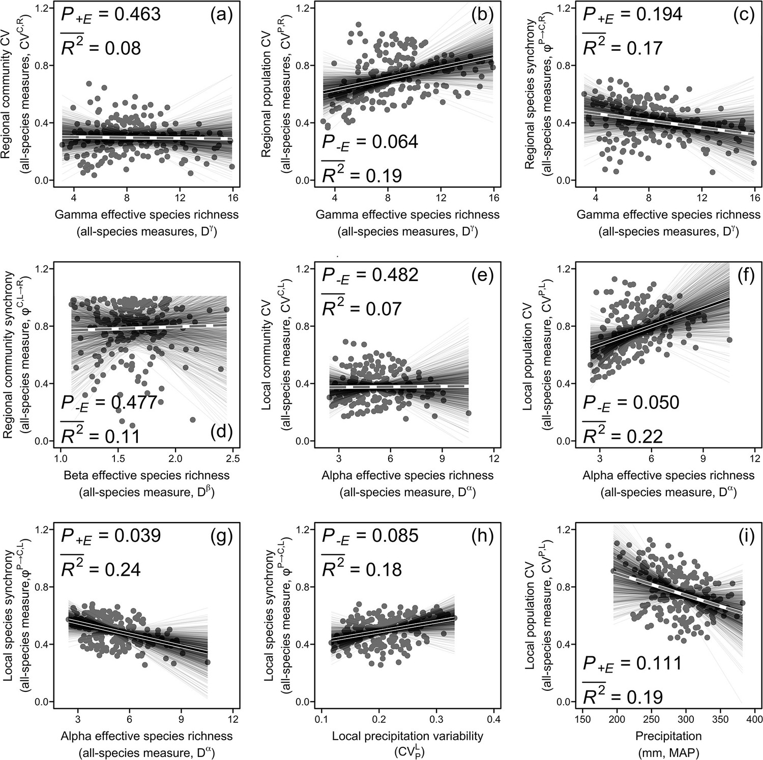
Regional community coefficient of variation (CV) (a), regional population CV (b), regional species synchrony (c), regional community synchrony (d), local community CV (e), local population CV (f), and local species synchrony (g) in relation to species diversity (effective species richness) as well as local species synchrony and local population CV, respectively, in relation to local precipitation variability (h) and precipitation (i) using all-species measures.
Solid black lines represent significant (p<0.05) and marginally significant (p<0.10) relationships, and dashed gray lines represent nonsignificant (p>0.10) relationships (see ‘Materials and methods’ for details and Box 1 for glossary). Thin grey lines represent relationships for 1000 sets of resampled regional communities (n=10 for each set). See Figure 4—figure supplement 1 for results of using dominant-species measures. Dataset and code are available in Figshare at https://doi.org/10.6084/m9.figshare.20281902.
Figure 4—figure supplement 1
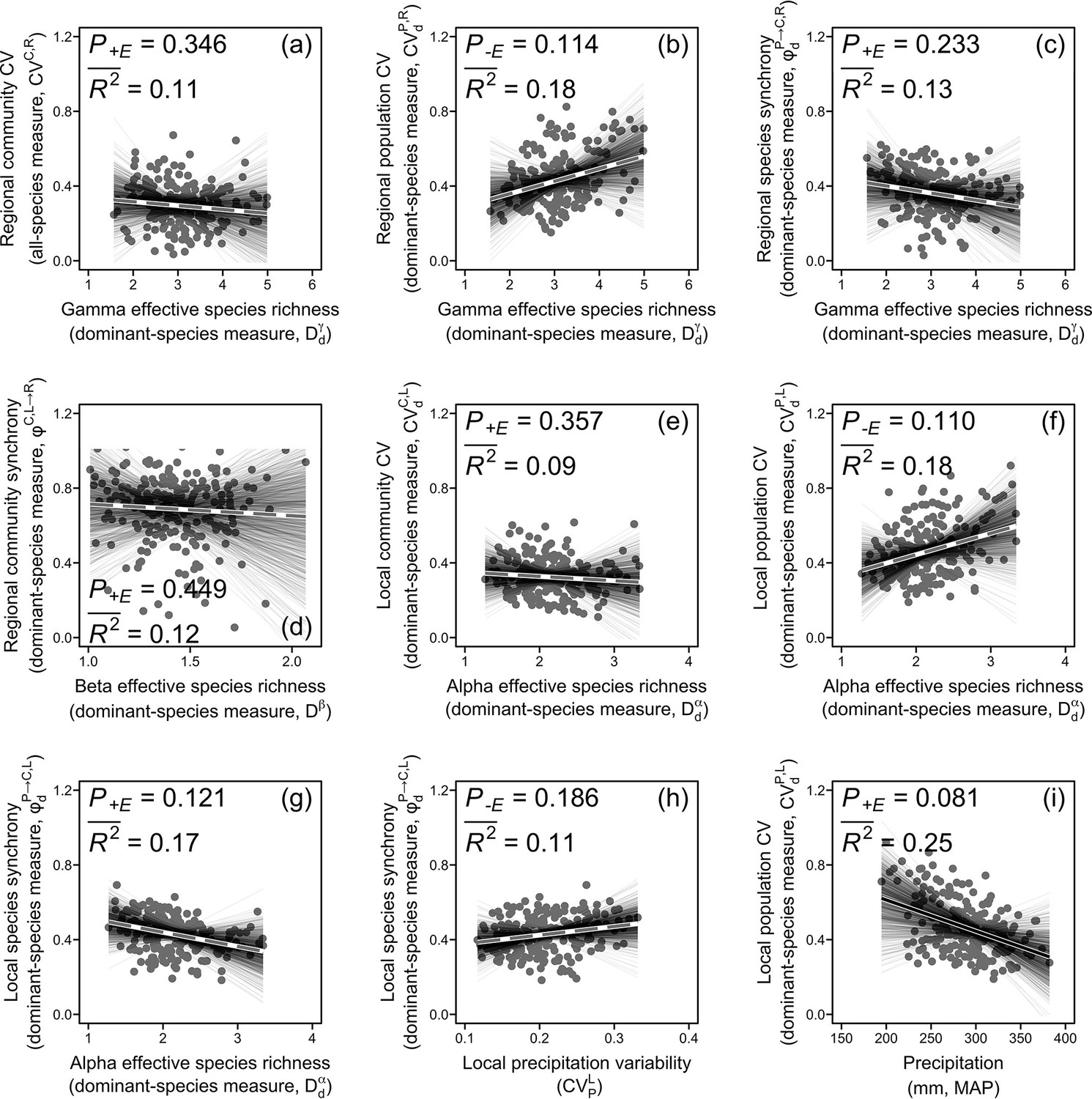
Regional community coefficient of variation (CV, inverse of stability) estimated with all species (a) and dominant-species estimates of regional population CV (b), regional species synchrony (c), regional community synchrony (d), local community CV (e), local population CV (f), and local species synchrony (g) in relation to species diversity (effective species richness) as well as dominant-species estimates of local species synchrony and local population CV in relation to local precipitation variability (h) and precipitation (i), respectively.
Solid black lines represent significant (P<0.05) and marginally significant (P<0.10) relationships and dashed grey lines represent non-significant (P>0.10) relationships (see ‘Materials and methods’ for details and Box 1 for glossary). Thin grey lines represent relationships for 1000 sets of resampled regional communities (n=10 for each set). Dataset and code are in Figshare at https://doi.org/10.6084/m9.figshare.20281902.
Appendix 1—figure 1

Time series of plant species biomass in each surveyed site.
Blue squares and lines represent species that only characterized as dominant species in local communities. Red diamonds and lines represent species characterized as dominant species in local communities and can also be characterized as dominant species when aggregating into regional communities. Green circles and lines represent subdominant species. It showed that most dominant species of local communities can be defined as dominant species of regional communities, with only a few exceptions. In addition, these species have higher productivity than others roughly all the time and are constantly exist in surveyed sites. Dataset and code are available in Figshare at https://doi.org/10.6084/m9.figshare.20281902.
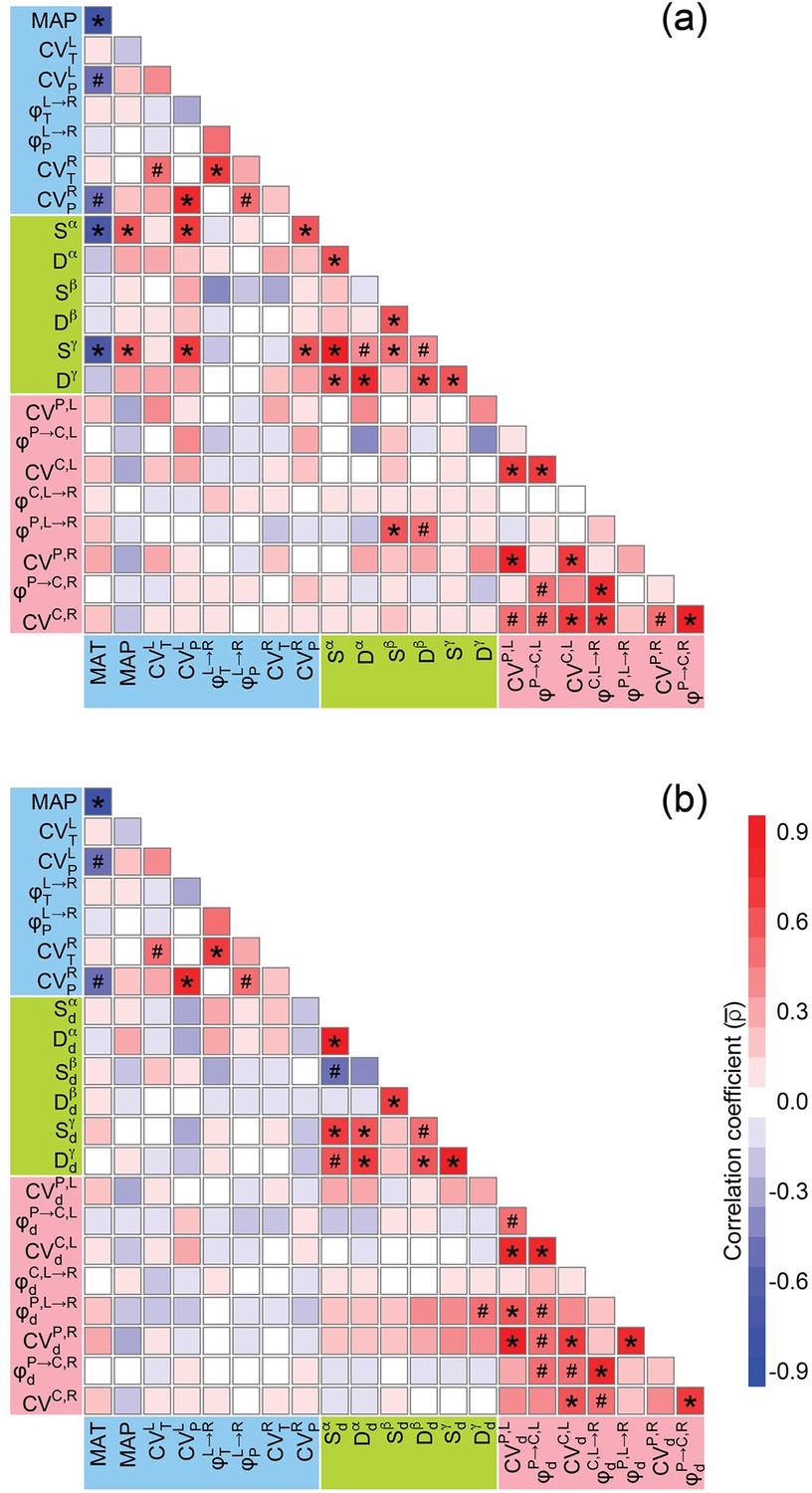
Appendix 1—figure 2
Correlation matrices for climatic factors, species diversity indices, coefficients of variation (CVs, inverse of stabilities), and synchronies (inverse of asynchronies) estimated with all species (a) and only dominant species (b) by considering a two-local-community scenario (see Figure 1b for a simplified case and Appendix 1—figure 3 for a three-local-community scenario).
Significant and marginally significant correlations are marked with *p<0.05 and #p<0.10, respectively (see ‘Materials and methods’ for details). Symbols and descriptions can be found in Box 1 and Appendix 1—table 1. Dataset, code, and relevant results are available in Figshare at https://doi.org/10.6084/m9.figshare.20281902.
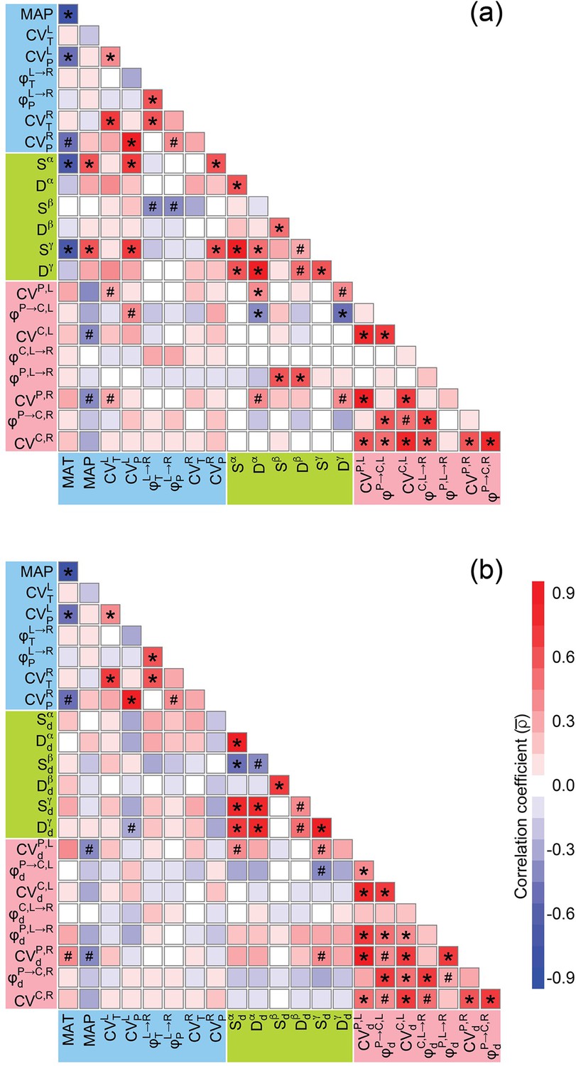
Appendix 1—figure 3
Correlation matrices for climatic factors, species diversity indices, coefficients of variation (CVs, inverse of stabilities), and synchronies (inverse of asynchronies) estimated with all species (a) and only dominant species (b) by considering a three-local-community scenario (similar sampling as in Figure 1b, but with three sites in each sample).
Significant and marginally significant correlations are marked with *p<0.05 and #p<0.10, respectively (see ‘Materials and methods’ for details). Symbols and descriptions can be found in Box 1 and Appendix 1—table 1. Potentially owing to the small sample size (n = 7) of the three-local-community scenario, many significant (or marginally significant) correlations found in the two-local-community scenario (n = 10, Appendix 1—figure 2) were nonsignificant for this three-local-community scenario. Thus, we did not further analyze the three-local-community scenario. Dataset, code, and relevant results are available in Figshare at https://doi.org/10.6084/m9.figshare.20281902.
Appendix 1—figure 4
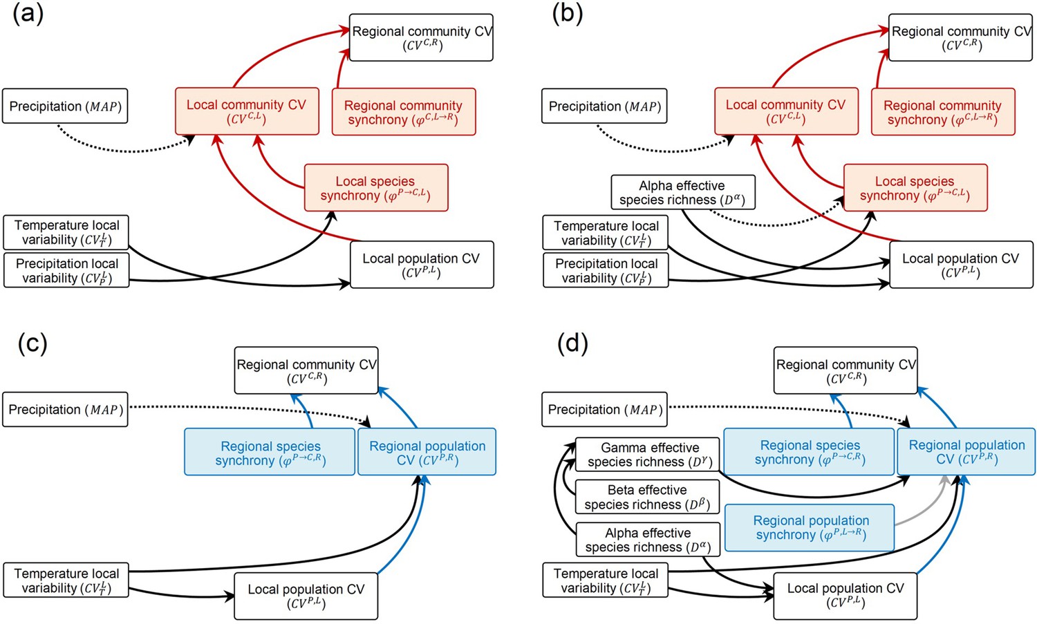
Initial path analysis models relating the regional community coefficient of variation (CV, inverse of stability) to its hierarchical components and species diversity indices estimated with all species as well as climatic factors according to the upscaling pathways of aggregating local communities (pathway I, a, b) or aggregating regional populations (pathway II, c, d).
Solid and dashed arrows represent significant (or marginally significant) positive and negative correlation relationships, respectively (Appendix 1—figure 2a). Gray solid arrow (regional population CV in relation to regional population synchrony), (d) represents nonsignificant positive correlation relationship, which is added in the initial model because it is theoretically proposed (Wang et al., 2019). Because (b) includes all paths of (a) and (d) includes all paths of (c), only the models shown in (b) and (d) are further analyzed (details are available in Figshare at https://doi.org/10.6084/m9.figshare.20281902). Symbols and descriptions can be found in Box 1 and Appendix 1—table 1.
Appendix 1—figure 5
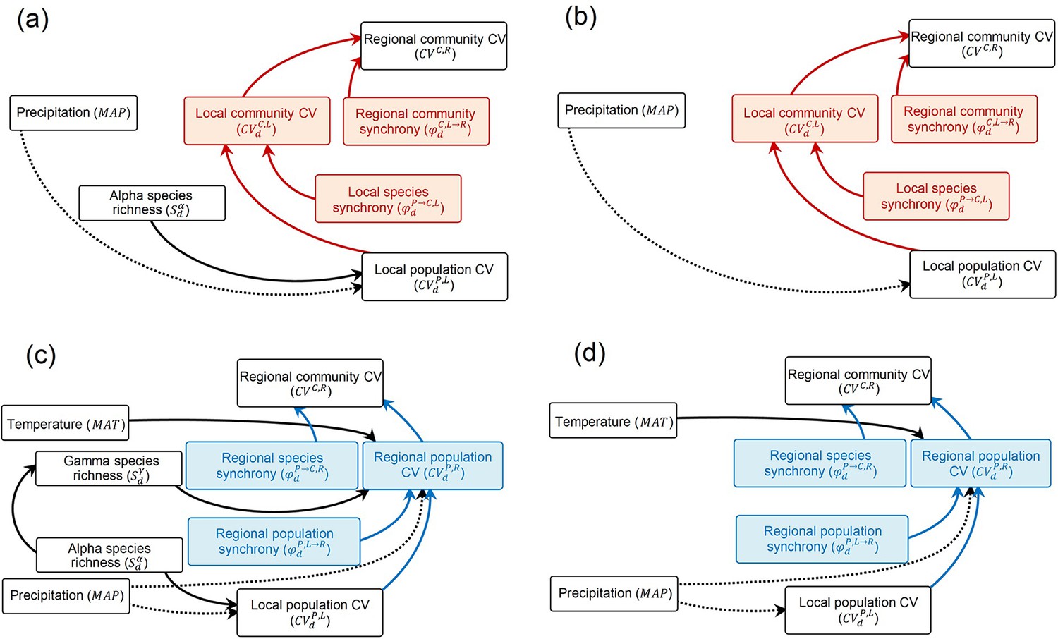
Initial path analysis models relating the regional community coefficient of variation (CV, inverse of stability) to its hierarchical components and species diversity indices estimated with only dominant species as well as climatic factors according to the upscaling pathways of aggregating local communities (pathway I, a, b) or aggregating regional populations (pathway II, c, d).
Solid and dashed color arrows represent significant (or marginally significant) positive and negative correlation relationships, respectively (Appendix 1—figure 2b). Because (a) includes all paths of (b) and (c) includes all paths of (d), only the models shown in (b) and (c) are further analyzed (details are available in Figshare at https://doi.org/10.6084/m9.figshare.20281902). Symbols and descriptions can be found in Box 1 and Appendix 1—table 1.
Author response image 1

Results of autocorrelation analyses for community productivity at each surveyed site.
Dashed lines indicate 95% confidence bands. There were no significant autocorrelations at any site.
Tables
Appendix 1—table 1
Notation summary for climatic factors, species diversity indices, coefficients of variation (CVs, inverse of stability), and synchronies (inverse of asynchrony) across spatial scales and hierarchical levels of ecological organization.
| Symbol | Description |
|---|---|
| Climatic factors | |
| MAT | Cross-site averaged mean annual temperature |
| MAP | Cross-site averaged mean annual precipitation |
| CVTL | Local CV of temperature |
| CVPL | Local CV of precipitation |
| φTL→R | Regional temperature synchrony |
| φPL→R | Regional precipitation synchrony |
| CVTR | Regional CV of temperature |
| CVPR | Regional CV of precipitation |
| Biodiversity indices | |
| Sα or Sdα | Alpha species richness estimated with all species or only dominant species |
| Sβ or Sdβ | Beta species richness estimated with all species or only dominant species |
| Sγ or Sdγ | Gamma species richness estimated with all species or only dominant species |
| Dα or Ddα | Alpha effective species richness estimated with all species or only dominant species |
| Dβ or Ddβ | Beta effective species richness estimated with all species or only dominant species |
| Dγ or Ddγ | Gamma effective species richness estimated with all species or only dominant species |
| Stability and synchrony | |
| CVP,L or CVdP,L | Local population CV estimated with all species or only dominant species |
| φP→C,L or φdP→C,L | Local species synchrony estimated with all species or only dominant species |
| CVC,L or CVdC,L | Local community CV estimated with all species or only dominant species |
| φC,L→R or φdC,L→R | Regional community synchrony estimated with all species or only dominant species |
| φP,L→R or φdP,L→R | Regional population synchrony estimated with all species or only dominant species |
| CVP,R or CVdP,R | Regional population CV estimated with all species or only dominant species |
| φP→C,R or φdP→C,R | Regional species synchrony estimated with all species or only dominant species |
| CVC,R or CVd_CC,R and CVd_PC,R | Regional community CV estimated with all species or only dominant species along pathways of aggregating local communities (pathway I: CVd_CC,R = φdC,L→R × CVdC,L) or organizing regional populations (pathway II: CVd_PC,R = φdP→C,R × CVdP,R) |
Additional files
Download links
A two-part list of links to download the article, or parts of the article, in various formats.
Downloads (link to download the article as PDF)
Open citations (links to open the citations from this article in various online reference manager services)
Cite this article (links to download the citations from this article in formats compatible with various reference manager tools)
Stability and asynchrony of local communities but less so diversity increase regional stability of Inner Mongolian grassland
eLife 11:e74881.
https://doi.org/10.7554/eLife.74881


