Parahippocampal neurons encode task-relevant information for goal-directed navigation
- Department of Neurobiology, Stanford University School of Medicine, United States
Figures
Figure 1 with 4 supplements
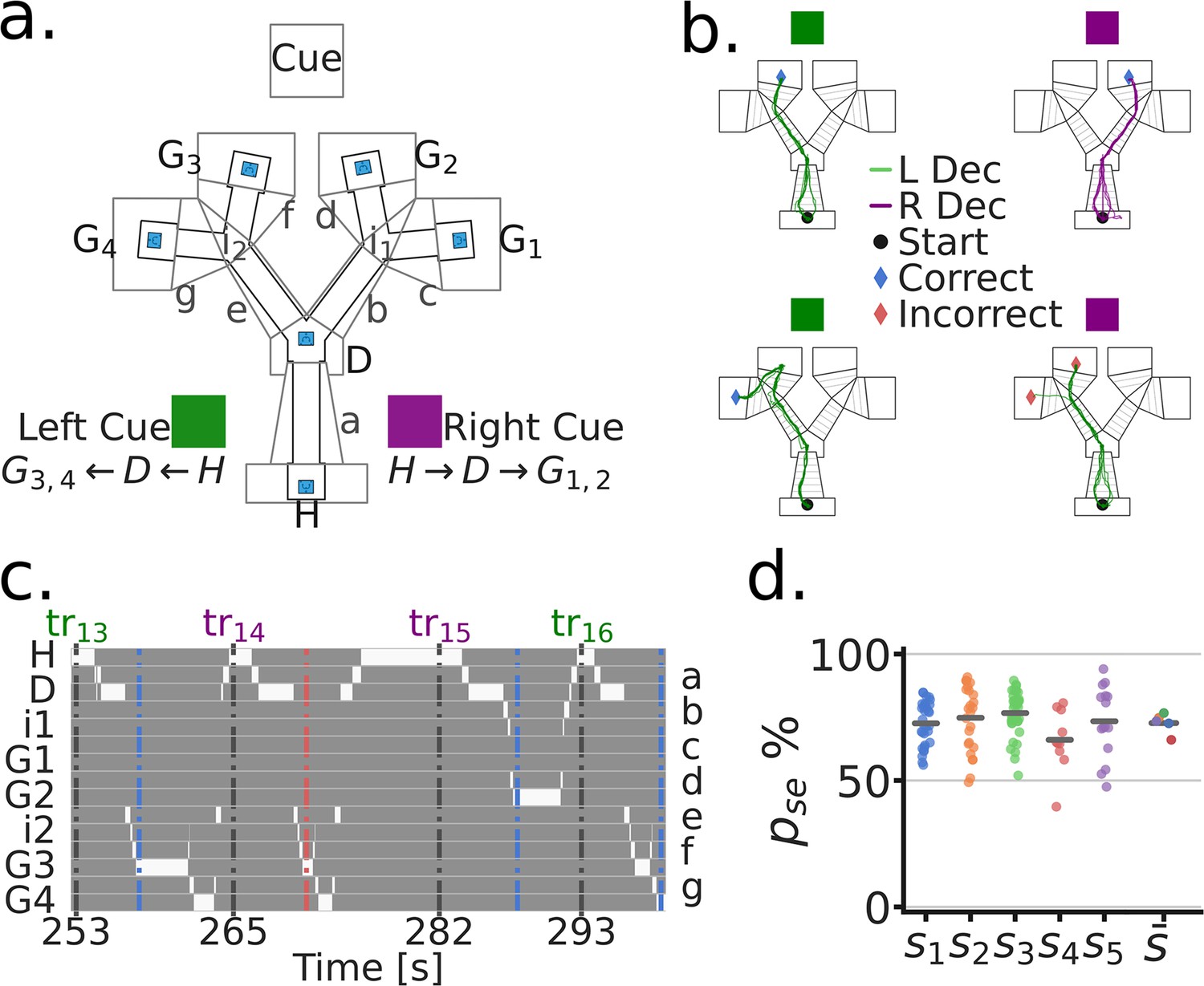
Goal directed navigation on the Tree-Maze task.
(a) Top view of the Tree-Maze layout and segmentation (indicated by upper and lower case letters) used for analyses (height = 1.4 m, width = 1.2 m). The LED cue panel was located at the end of the maze (flattened for illustration). Colored cue cards on the side of the maze indicate the two cue types by trial (Purple = Right Cue [RC], Green = Left Cue [LC]). Possible reward locations denoted by capital letters (Home = H, Decision = D, Goal = G1 G4). Lower case letters correspond to the segments shown on the right side of panel c. Reward wells highlighted in blue. (b) Colored lines indicate example trajectories of a rat, five trials per panel. L Dec indicates a trajectory towards the left branch and R Dec indicates a trajectory towards the right branch. Left column (Left/Green cue), trajectories to G3 (top) and G4 (bottom) for reward. Both of these were correct navigational decisions and were rewarded. Right column (Right/Purple cue), trajectories to G2 (top) and G3 (bottom), only the top trajectories resulted in reward at a goal. (c) Binary trajectory segmentation time window. At any given time-point, the subject can only be at one location in the maze (indicated by the white bins). Bottom axis indicates trial start times (seconds). Top axis indicates the trial number (tr), colored coded by cue. Left/Right axis indicates the identity of the segment, lower case letters on the right correspond to those in panel a. Blue and red dashed vertical lines indicate the end of a trial (blue = correct; red = incorrect). (d) Task performance by subject. Each dot corresponds to a session by subject. For , dots indicates the subject mean. = performance in a session.
Figure 1—figure supplement 1
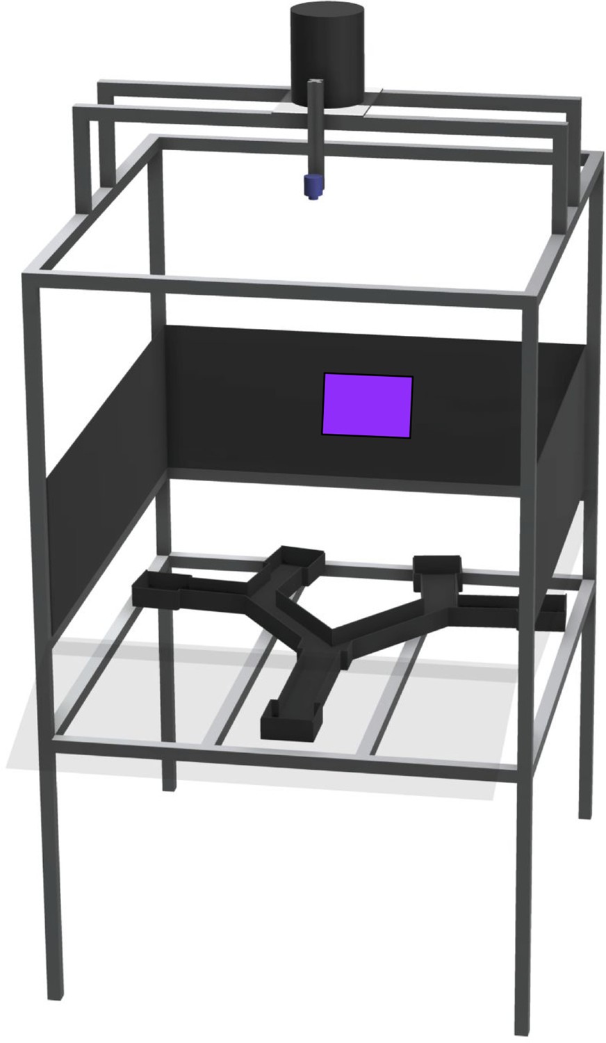
Data collection and behavior apparatus.
An aluminum frame housed both the open-field arena and Tree-Maze maze. The open-field ‘floors’ were easily swapped in for open-field recordings, or taken out for Tree-Maze recordings. The height difference between the two was 0.35 m, with all other peripheral cues staying constant across recording types. LED panel shown in purple at the back of the maze represents the ‘Right Cue’.
Figure 1—figure supplement 2
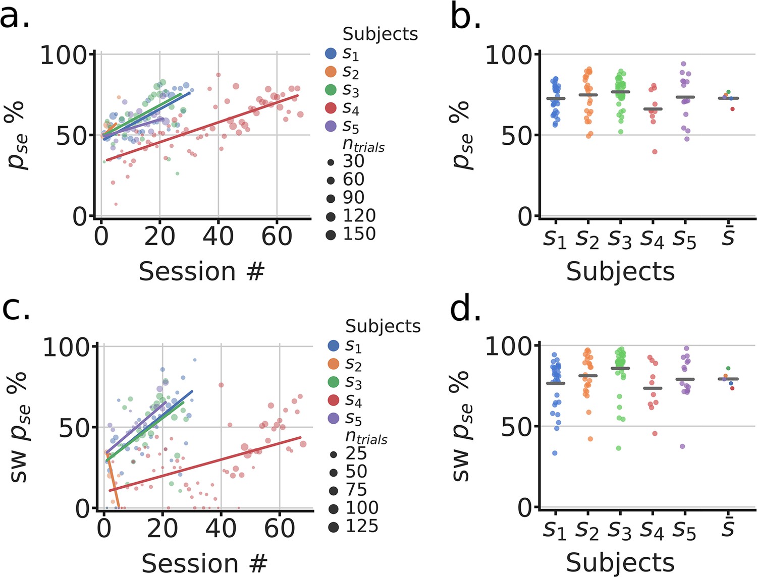
Subject learning and post-surgery behavior.
(a) Tree-Maze performance by training session until performance criteria was reached (# trials = 80, ). Each dot corresponds to the performance on a given session, with colors identifying subjects and dot size indicating the number of trials in the session. Lines correspond to least squares regression by subject. (b) Subject performance on the Tree-Maze task, post-surgery (Same as Figure 1d). Neural recordings were performed during all of these sessions. (c, d) Same as (a) and (d), respectively, but for performance on switch trials.
Figure 1—figure supplement 3
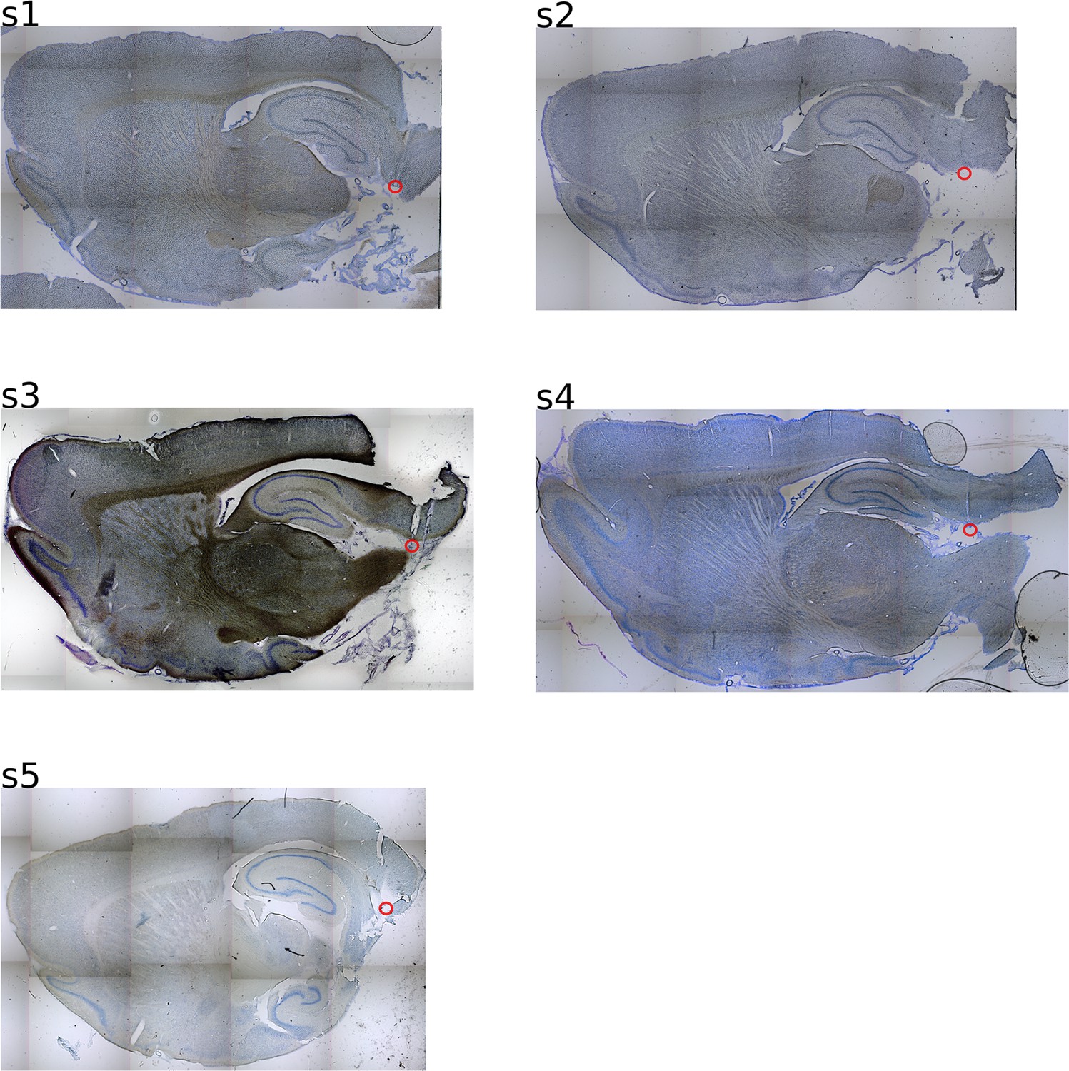
Sagittal histology sections illustrating the location of recording electrodes.
Coordinates for tetrode implantation ranged from 1 to 4 mm from the corital surface, 7.5–9 mm from bregma (anterior-posterior) and 3.6–4.6 mm from the midline (medial-lateral). Drive-able tetrodes with protective tubing were used and estimated end position highlighted with red circles. Tissue damage prohibited accurate localization of recording locations, with estimates being mostly MEC with some PaS and PrS.
Figure 1—figure supplement 4
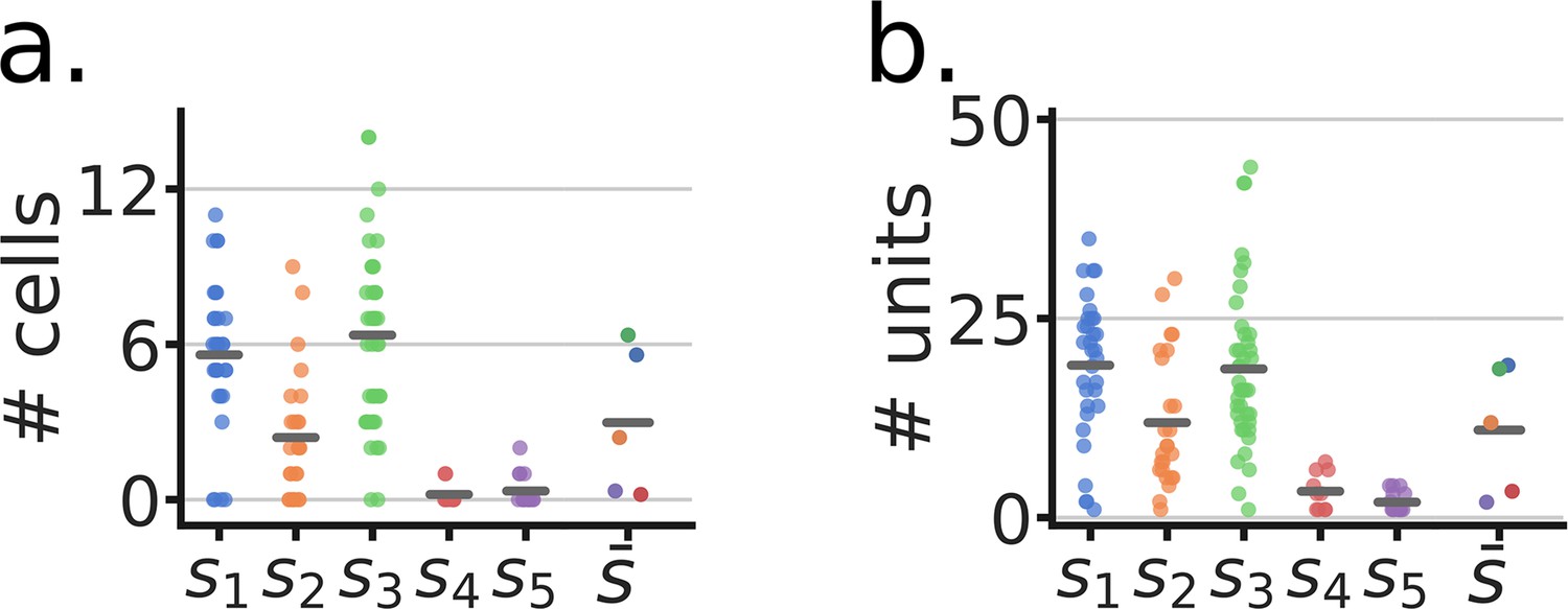
Number of units by session and subject.
(a) Putative isolated units by subject. Each dot is a recorded session and horizontal bars indicate the mean by subject. The indication of corresponds to subject means, color coded corresponding to each subject. (b) Same as (a) but with the inclusion of MUA.
Figure 2 with 7 supplements
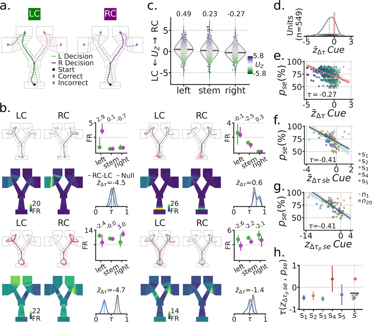
Spatial remapping was associated with the visual cue and correlated with task performance.
(a) Example session trajectories for all LC (Left-Cue) and RC (Right-Cue) trials. (b) Four example single-units. For each example unit: Top row, left and middle, outbound trajectories separated by cue (red dots = spikes). Top-right, trial median activity by cue and maze segment (left, stem, right), numbers at the top indicate the Mann-Whitney Z transformed U statistic for the difference between the RC and LC trial distributions . Bottom row, mean spatial rate maps by zone and cue, color coded for minimum (firing rate [FR]=0, blue) and maximum (yellow) values. Bottom right, re-sampled distribution of correlations between RC and LC maps in blue for that unit, and in grey the corresponding null distribution. Remapping score is the mean remapping score for each unit. (c) Distributions of scores for all recorded units by maze segment. Purple means higher FR for RC than LC, Green means higher FR for LC than RC. Note the higher FR for RC on the left segment (far left) and higher FR for the LC on the right segment (far right). (d) Distribution of mean remapping scores by unit, note the negative shift in the distribution of scores. (e) Scatter-plot between the task performance on a given session and the cue remapping scores for recorded units in that session. Size and color of dots scale with the x axis for illustration. Regression line in red with a band. Kendall correlation score between behavior and remapping score shown. (f) Scatter-plot between and the mean remapping score across units recorded in a given session . Size of dots indicate number of co-recorded units, color codes correspond to different subjects. Regression line and corresponding band shown in grey. (g) Like (f) but with neural population correlation, composed of the spatial rate maps for all recorded units in a session. (h) Correlation between and by subject, with bootstrapped standard deviation (B=500). is the across subject mean.
Figure 2—figure supplement 1
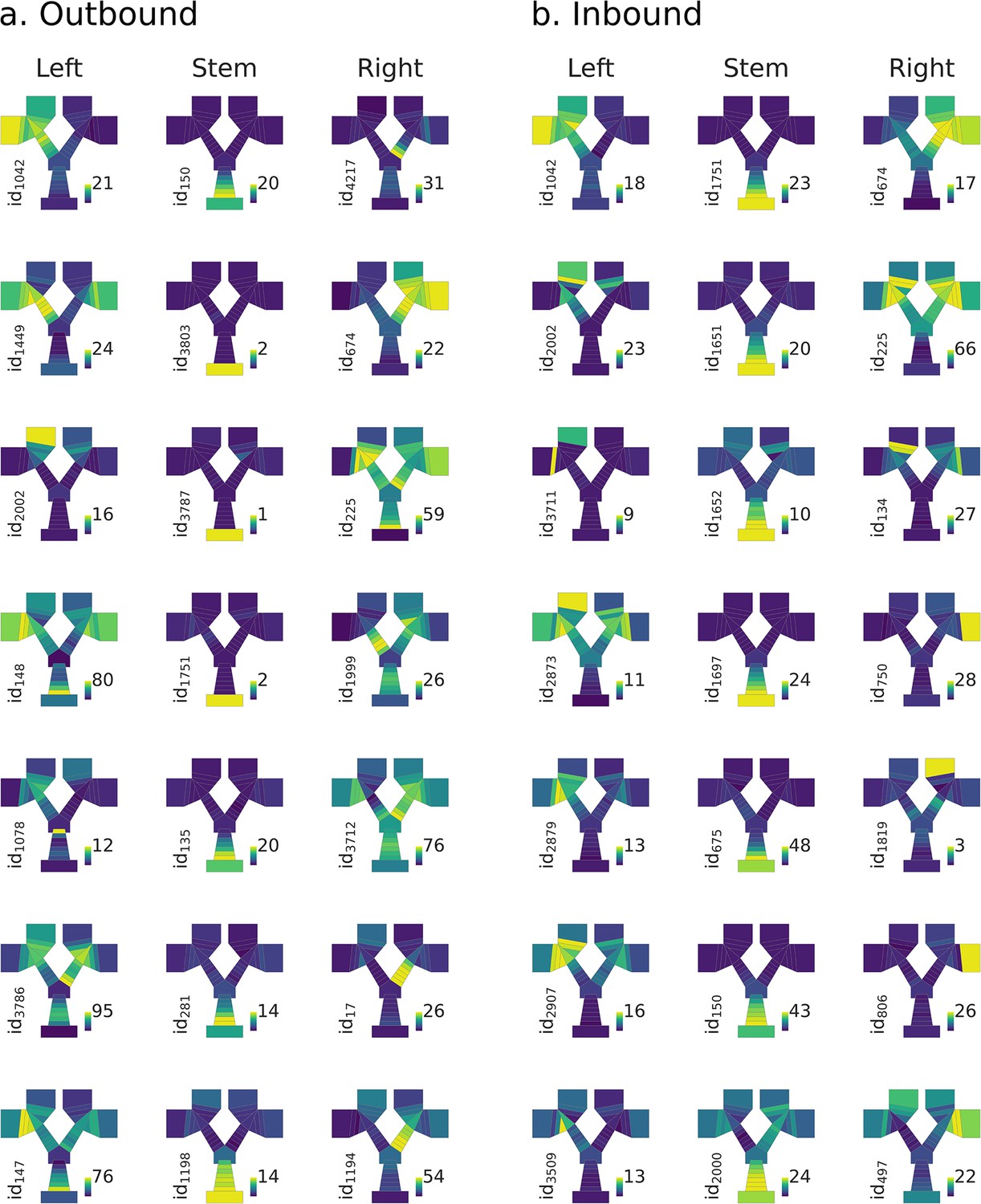
Example rate maps of segment selective units.
Units ranked (from top to bottom), by taking the Mann-Whitney statistic of that segment vs the two other segments (e.g. activity on Left vs activity on Stem and Right). (a-b) Outbound trajectories (a) and inbound trajectories (b). Note that there is some overlap in selected units for inbound and outbound, indicating position tuning that was not directional.
Figure 2—figure supplement 2
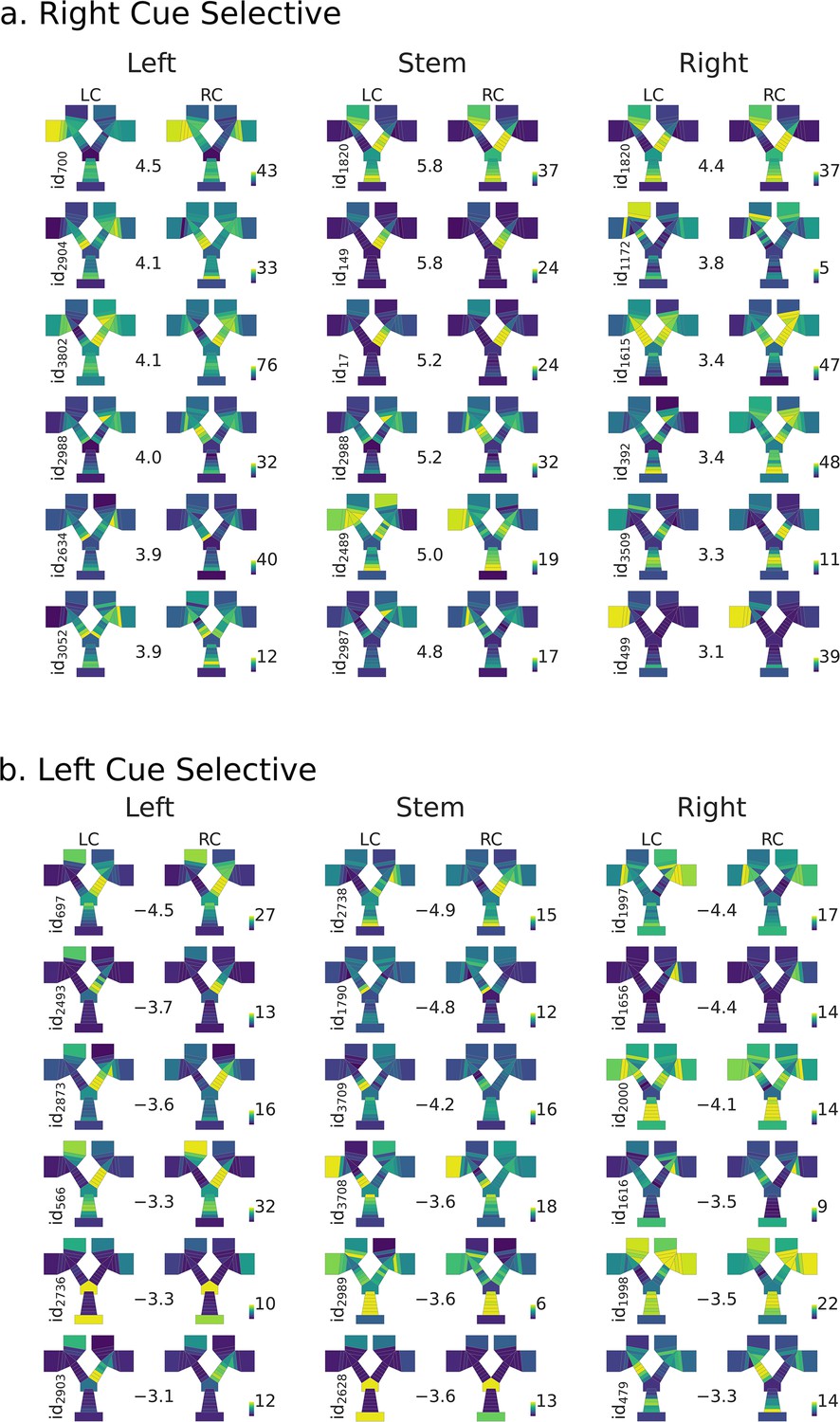
Spatial rate maps of cue selective units.
Units ranked (from top to bottom) by taking the Mann-Whitney statistic by segment of Right-Cue vs Left-Cue outbound trial conditions, statistic shown between each pair of rate maps. Columns refer to which segment of the maze was selected (left, stem, right). Rate maps are generated by averaging the activity by condition. Units shown were selected based on ranking of all the units according to the statistic value. The 90% of the max firing rate (spikes/second) of each pair of rate maps is shown in colormap, with all colormaps being referenced to 0 spikes/second. (a) Spatial rate maps of right cue selective units by segment. Note that all values are positive. (b) Spatial rate maps of left cue selective units by segment, all values are negative.
Figure 2—figure supplement 3
Unit examples of stronger cue coding while in the incorrect branch.
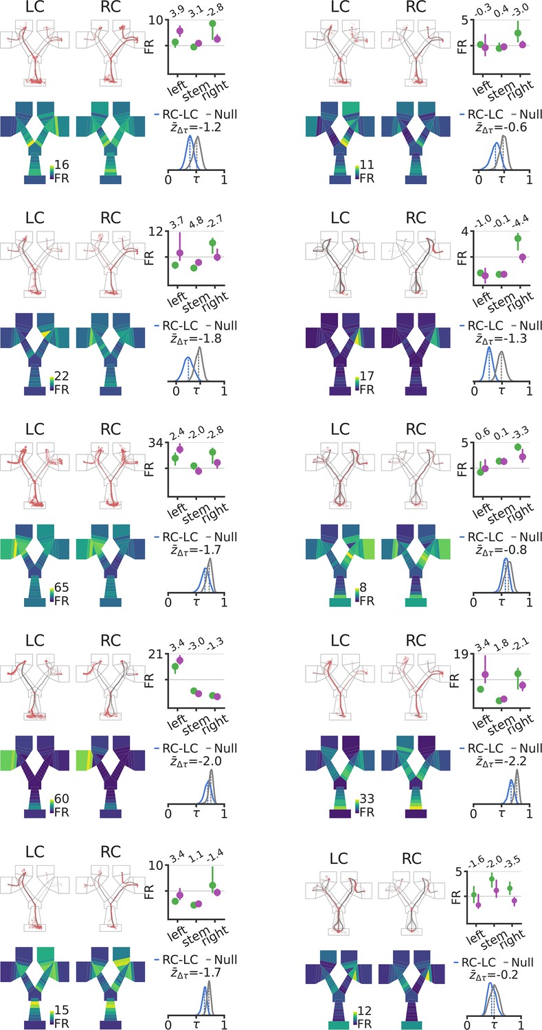
Selection of units based on stronger coding for Left-Cue than Right-Cue when in the right branch of the maze, or stronger coding for Right-Cue than Left-Cue when in the left branch of the maze. Ten units, with each unit block showing raw spike/trajectories, rate maps, firing rate by segment x cue, and remapping distribution (as in Figure 2).
Figure 2—figure supplement 4
Incorrect coding in mean firing rates.
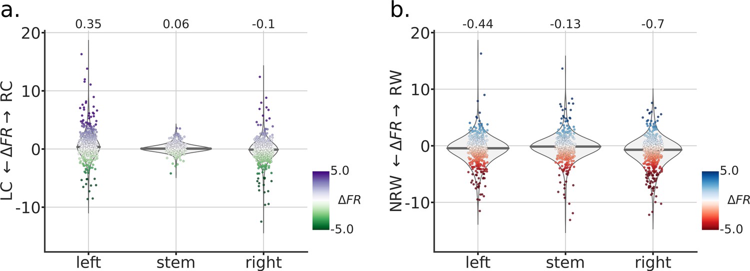
(a) Plotted as in Figure 2c, with values being the difference of mean firing rates by cue condition and by maze segment. Even in this un-normalize space, the results follow what is reported in the main text. (b) Plotted as in Figure 4c, with values being the difference of mean firing rates by reward condition and by maze segment.
Figure 2—figure supplement 5

Incorrect coding in Z-scored firing rates.
(a) Z-scored firing rate of all units by cue and maze segment. Individual unit color codes: Purple (CR >CL) and Green (CL >CR). Dot-lines are the averages for each of groupings. Note more ‘Purple’ in the left segment of the maze and more ‘Green’ in the right segment. Analysis is for illustration only as the pre-allocation of units to groups biases any analyses. (b) Mean activity of all units by cue and maze segment (N=549). Note that all the general patterns of ‘error’ / ‘incorrect’ coding are as in the main analyses. (c) Mean activity by subject. We replicate the above results by first taking the mean activity across each subject’s units by cue and maze segment. Note that all the patterns are as in the main analyses.
Figure 2—figure supplement 6

Cue remapping vs behavior control analyses for isolated units.
(a) Original results as reported in Figure 2. Top-left, distribution of remapping scores across units. Bottom-left, session performance by remapping score for each unit. Color and size of dots scale with x-axis. Red line is the robust regression line with 95% confidence band. Kendall between the quantities reported in the graph. Top-right, each dot is the average remapping score by session (color = subject, size = # of units in the average). Robust regression and 95% confidence band shown in dark blue. Bottom-right, each dot is the population correlation for the session. (b-d) Positive control analyses, same as (a). (b) Use of Pearson correlation instead of Kendall correlation to compute the remapping score. (c) Each period post 500ms of reward delivery is removed from the analyses, avoiding possible artifacts due to activation of reward pump. (d) Each period of speed being less than 2 cm/s is removed from the analyses, only mobility periods go into the analyses. For all control analyses, we observed a significant relationship between remapping and behavior.
Figure 2—figure supplement 7
Cue remapping vs behavior control analyses for isolated units and MUA.
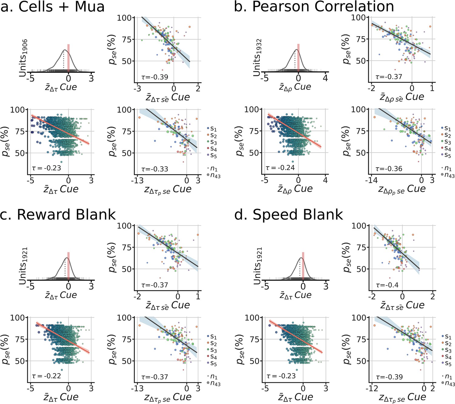
Panels follow convention in Figure 2—figure supplement 6. (a-d) Top-left, distribution of remapping scores across units. Bottom-left, session performance by remapping score for each unit. Color and size of dots scale with x-axis. Red line is the robust regression line with 95% confidence band. Kendall between the quantities reported in the graph. Top-right, each dot is the average remapping score by session (color = subject, size = # of units in the average). Robust regression and 95% confidence band shown in dark blue. Bottom-right, each dot is the population correlation for the session (including both isolated units and MUA). (b) Use of Pearson correlation instead of Kendall correlation to compute the remapping score. (c) Each period post 500ms of reward delivery is removed from the analyses. (d) Each period of speed being less than 2 cm/s is removed from the analyses. For all control analyses, we observed a significant relationship between remapping and behavior.
Figure 3 with 1 supplement
Cue modeling revealed rate remapping and trial-wise correlations to behavior.
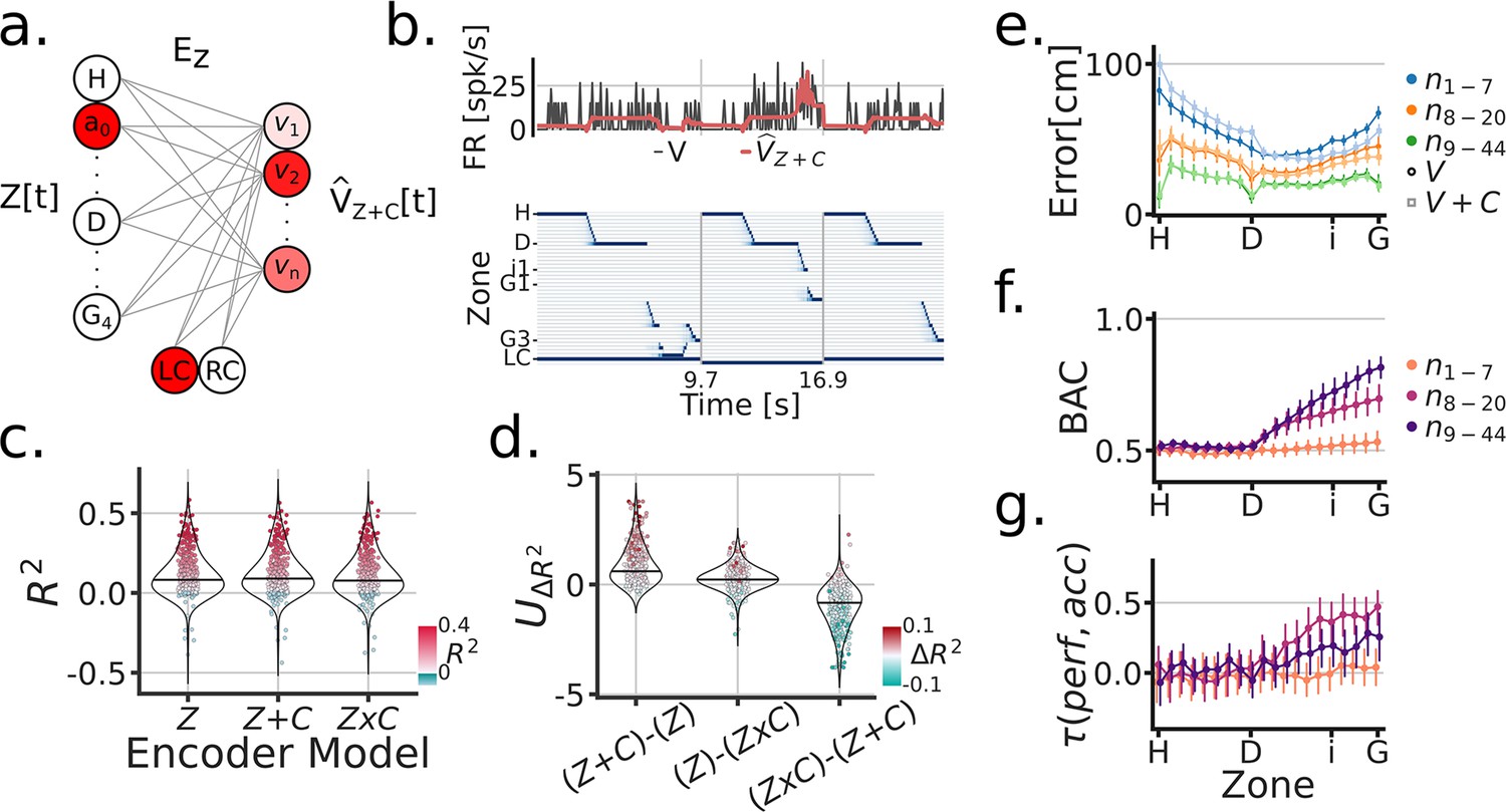
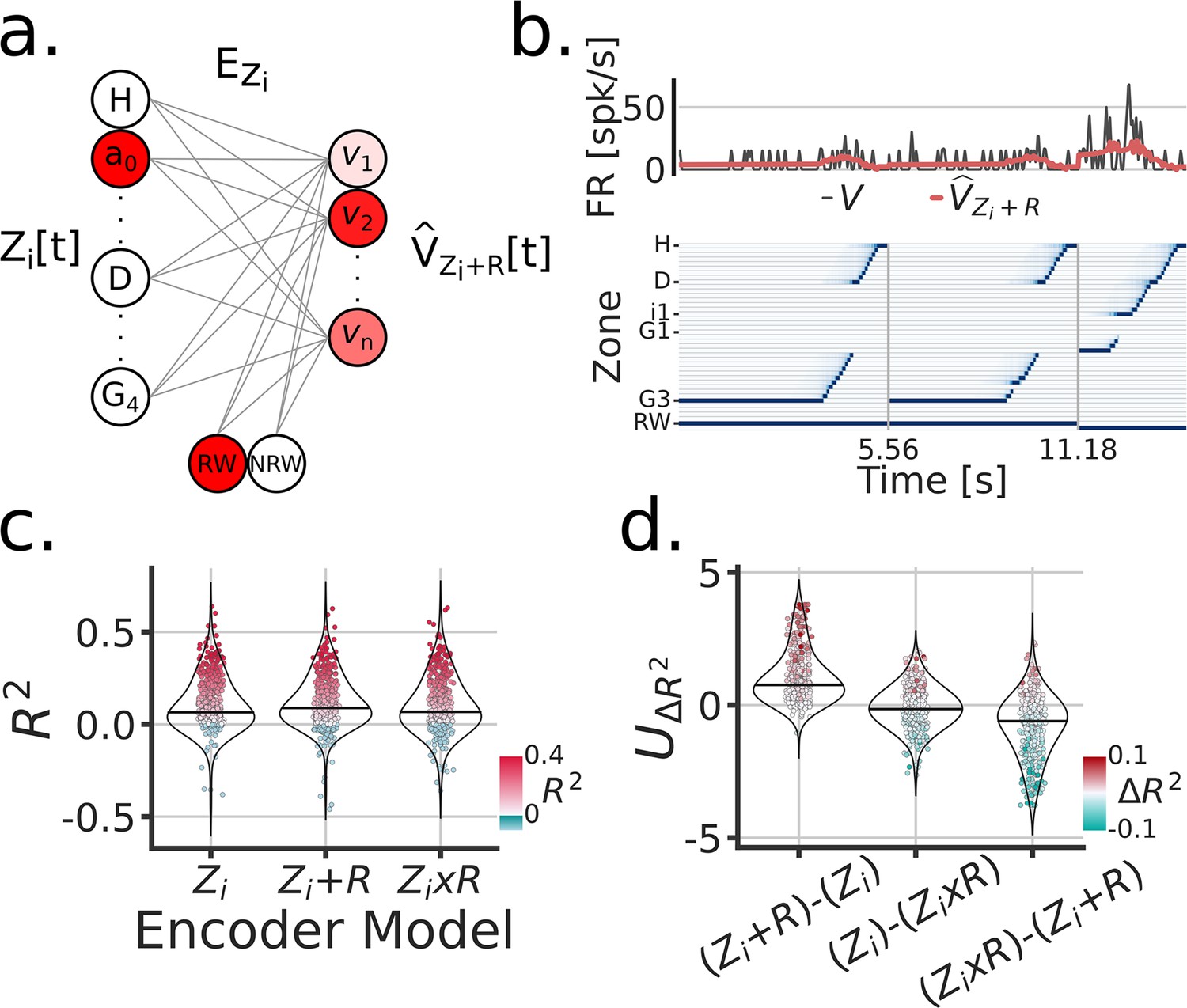
(a) Linear zone encoding model with cue , at a given sample time , the current position of the animal and the cue identity is multiplied by learned weights to predict FR for each recorded unit . (b) Example time window of , the true FR in black and the predicted FR in red . (c) Model comparison between three types of zone encoding: only zones, zones + cue, a set of zones for each cue. Each dot is a unit, blue dots were negative , red scales with and y-axis. (d) Model comparison scores. Y-axis is the Mann-Whitney Z transformed statistic for comparing the on test folds. Colorbar indicates the median difference in across test folds. (e) Performance of linear zone decoder models (circles) and (squares). Y-axis is the error distance in cm between the predicted and true zone, X-axis is the linearized Tree-Maze zones displayed as H (Home-well) to D (Decision-well) to i (second intersection/branching) to G (Goal-well). Linearization achieved through averaging the equivalent trajectories towards the goal. The hue shade provides groupings of sessions according to number of co-recorded units (both isolated an MUA included in these analyses). (f) Performance of linear decision decoder by zone, with color indicating number of units. Note the sharp decision well split in the performance. BAC = balanced accuracy. (g) Correlation between the subject’s performance and the model by zone. Color groupings as in (f). Model performance is the comparison between the output of the decision decoder and the true identity of the cue, the same computation used to assess a subject’s performance.
Figure 3—figure supplement 1
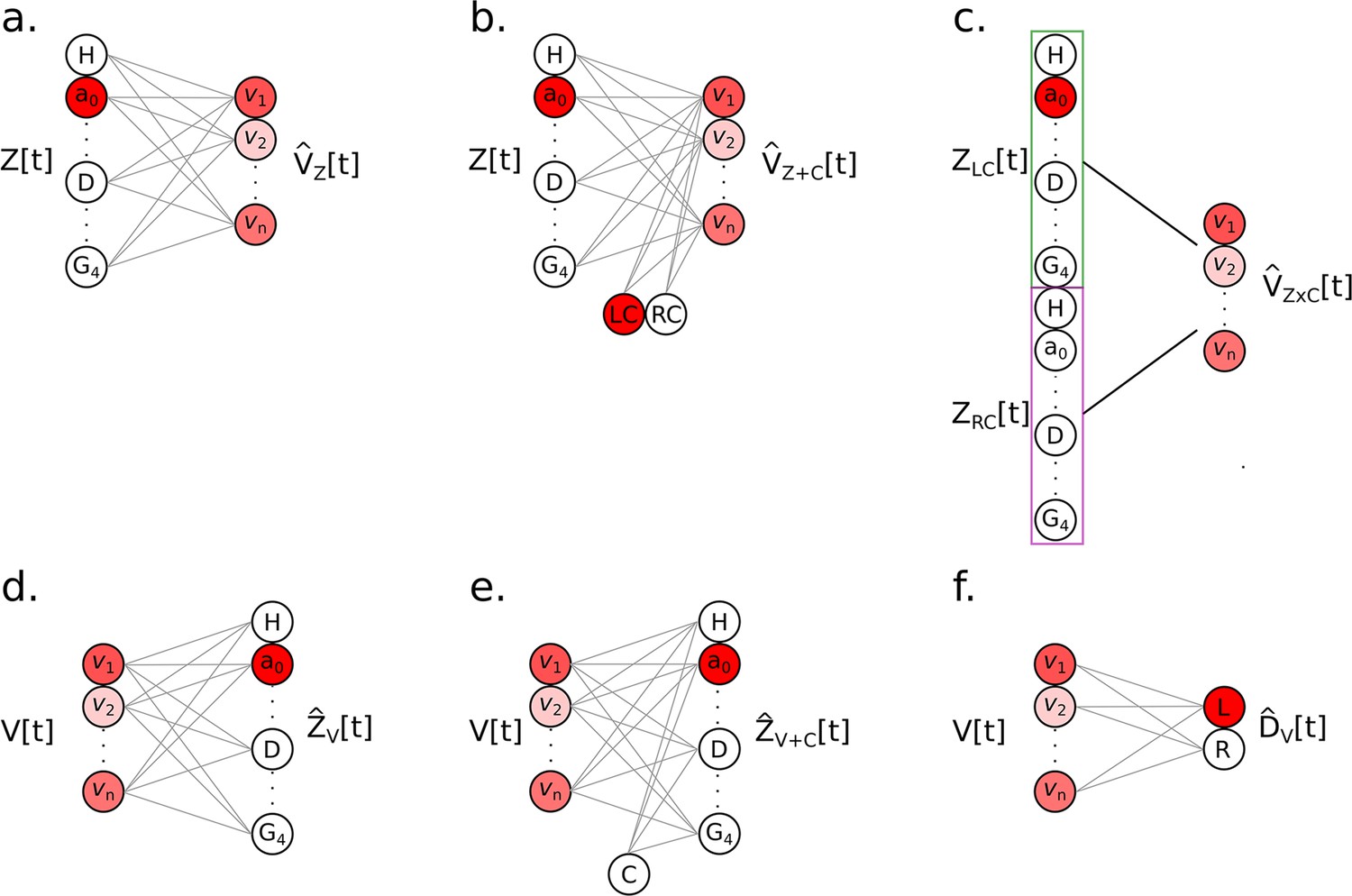
Encoder and decoder model diagrams.
(a) Zone encoder model, , that uses the position of the animal at time [t] to predict the neural activity after a linear transformation. Note that only one zone can be active at a time. Intensity of red color indicates activity. (b) Zone encoder plus cue identity model (, rate-remapping model). Note that only one cue can be active by trial, effectively functioning as a single modulatory gain signal that would change the activity across the trial duration. (c) Zone encoder by cue identity model (, global-remapping model). This model had two sets of positions, with only one set active as a function of cue, effectively allowing for completely orthogonal maps to be used to predict the neural activity. Position sets indicated by color. Reward encoding models followed the same convention, with RW instead of cue. (d) Zone decoder model that uses the neural activity to predict the subject’s position, . Omitted from the diagram is the presence of a softmax normalization that produces probability values for each zone. The maximum probability at a given time is used as the prediction of position for that time. (e) Zone decoder model, like (d), plus the inclusion of cue information . Note that a weighted cue value is added to neural activity by zone, before the softmax operation. This approach thus allow the cue to have different effects by zone. (f) Decision decoder, , that uses neural activity to predict the subject’s decision (Left/Right) by time. Omitted from the diagram is the cumulative temporal integration of predictions by trial, allowing the decoder to accumulate evidence as the subject traverses the maze.
Figure 4 with 7 supplements
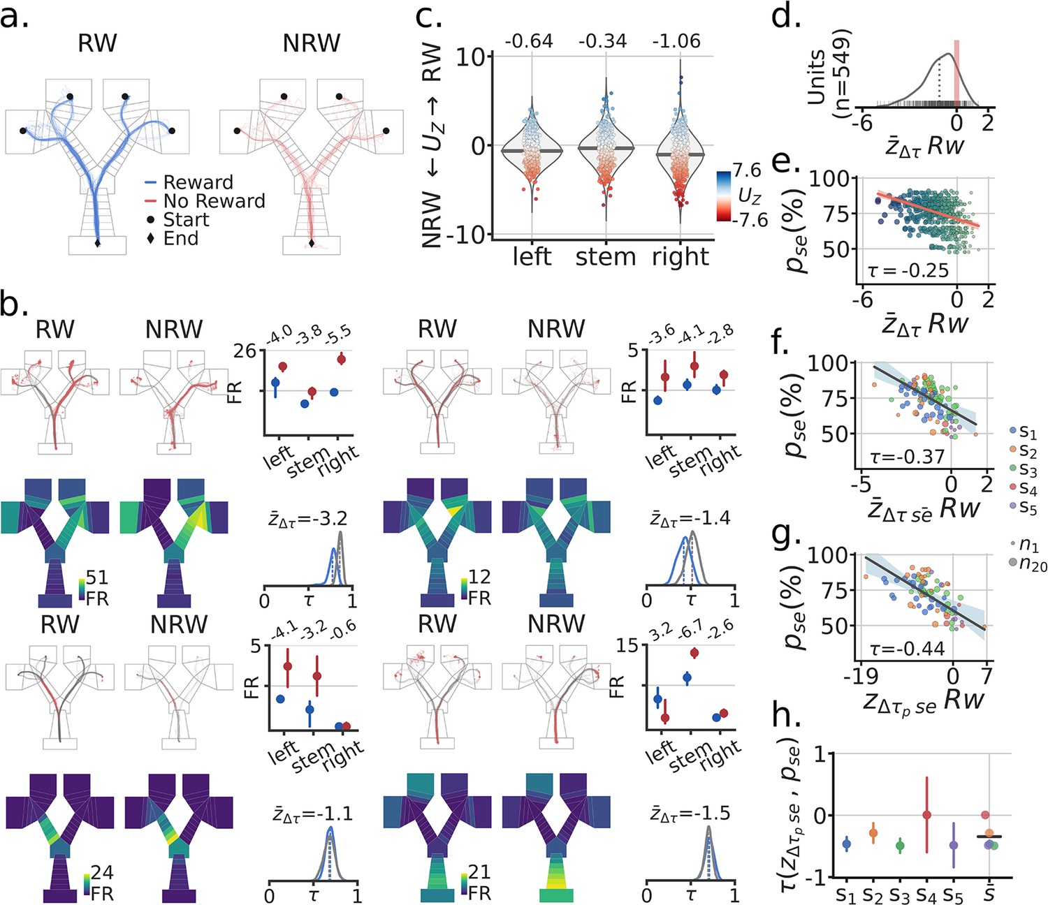
Absence of reward leads to higher activity and spatial remapping.
(a) Example session RW (reward) and NRW (no-reward) trials. (b) Four example units (i–iv). Top rows, inbound trials trajectories by RW/NRW (red dots = spikes). Top-right, trial median activity by RW and segment in the maze. Firing rate difference score as described in the main text. Bottom rows, mean spatial rate maps by zone and RW, minimum FR = 0. Bottom right, re-sampled distribution of correlations between RW and NRW maps in blue for that unit, and in grey the corresponding null distribution. Remapping score is the mean remapping score for each unit. b.i Session is the same as in panel a., other units from different sessions. (c) Distributions of scores for all recorded units by maze segment. Blues means higher FR for RW than NRW trials, Red higher NRN than RW. (d) Distribution of mean remapping scores by unit, note the negative shift in the distribution of scores. (e) Scatter-plot between a session’s task performance and the remapping scores for recorded units. Size and color of dots scale with the x axis for illustration. Regression line in red with a band. Kendall correlation score between behavior and remapping score shown. (f) Scatter-plot between and the mean remapping score across a sessions units . Size of dots indicate number of co-recorded units, color codes correspond to different subjects. Regression line and corresponding band shown in grey. (g) Like (f) but with neural population correlation, composed of the spatial rate maps for all recorded units in a session. (h) Correlation between and by subject, with bootstrapped standard deviation (B=500). is the across subject mean.
Figure 4—figure supplement 1
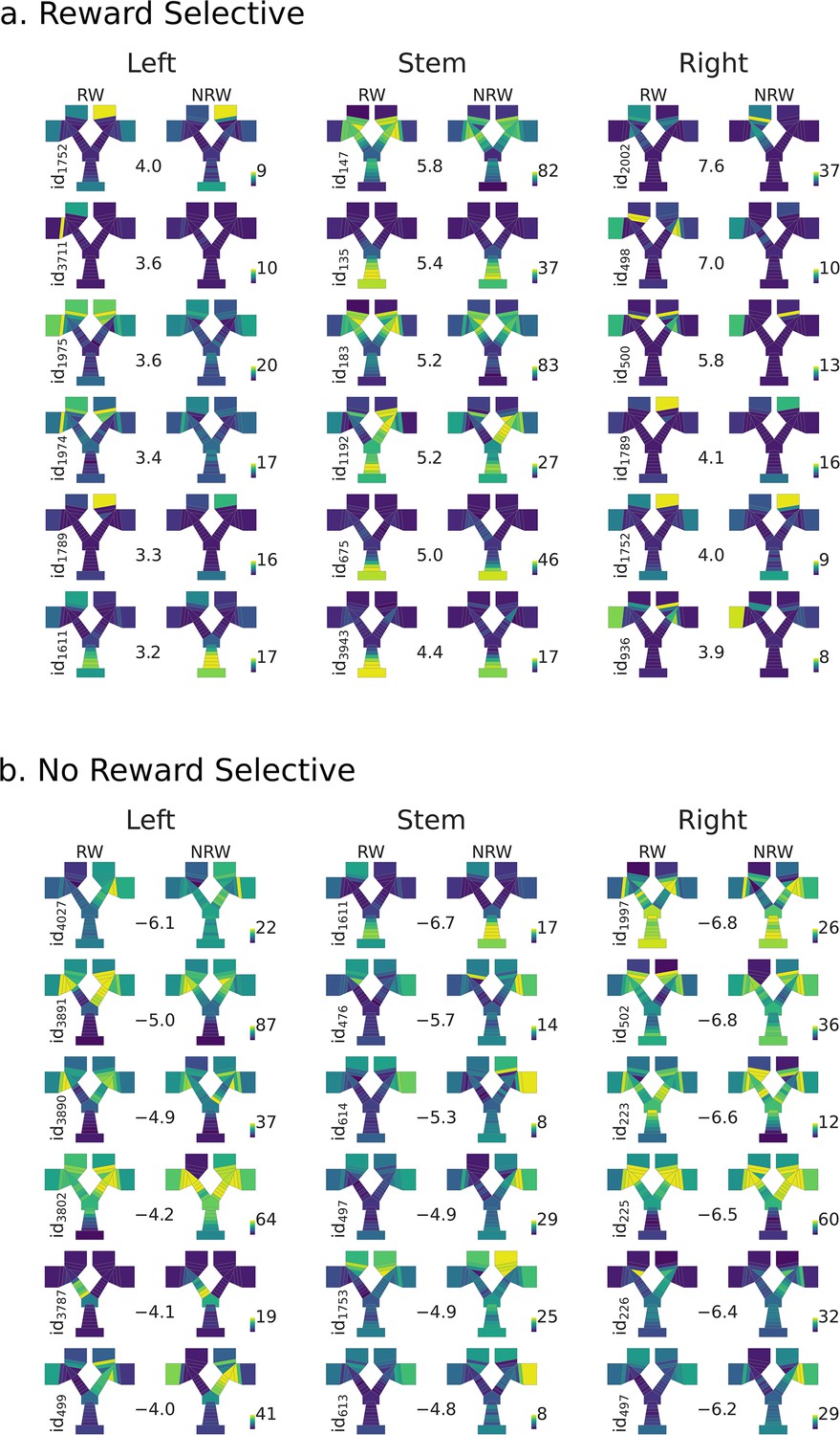
Spatial rate maps of reward selective units.
Units ranked (from top to bottom) by taking the Mann-Whitney statistic by segment of reward vs no-reward inbound trials conditions, statistic shown between each pair of rate maps. Columns refer to which segment of the maze was selected (left, stem, right). Rate maps are generated by averaging the activity by condition. Units shown were selected based on ranking of all the units according to the statistic value. The 90% of the max firing rate (spikes/second) of each pair of rate maps is shown in colormap, with all colormaps being referenced to 0 spikes/second. (a) Spatial rate maps of reward selective units by segment. Note that all values are positive. (b) Spatial rate maps of no-reward selective units by segment, all values are negative.
Figure 4—figure supplement 2

Spatial rate maps of direction selective units.
Units ranked (from top to bottom) by taking the Mann-Whitney statistic by segment of outbound vs inbound trajectories for all trials, statistic shown between each pair of rate maps. Rate maps are generated by averaging the activity by condition. Units shown were selected based on ranking of all the units according to the statistic value. The 90% of the max firing rate (spikes/second) of each pair of rate maps is shown in colormap, with all colormaps being referenced to 0 spikes/second. (a) Spatial rate maps of outbound selective units by segment. Note that all values are positive. (b) Spatial rate maps of inbound selective units by segment, all values are negative.
Figure 4—figure supplement 3
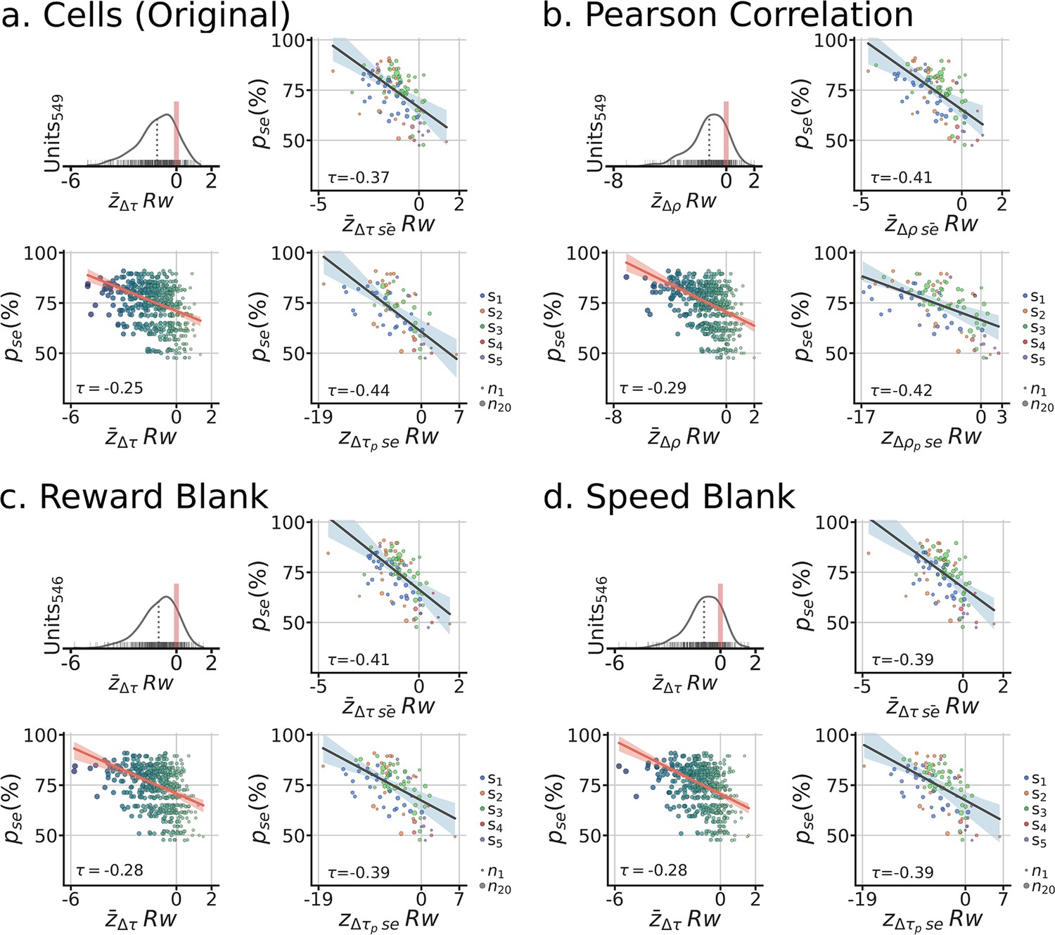
Reward remapping vs behavior control analyses for isolated units.
Panels follow convention in Figure 2—figure supplement 6. (a-d) Top-left, distribution of remapping scores across units. Bottom-left, session performance by remapping score for each unit. Color and size of dots scale with x-axis. Red line is the robust regression line with 95% confidence band. Kendall τ between the quantities reported in the graph. Top-right, each dot is the average remapping score by session (color = subject, size = # of units in the average). Robust regression and 95% confidence band shown in dark blue. Bottom-right, each dot is the population correlation for the session. (b) Use of Pearson correlation instead of Kendall correlation to compute the remapping score. (c) Each period post 500ms of reward delivery is removed from the analyses. (d) Each period of speed being less than 2 cm/s is removed from the analyses. For all control analyses, we observed a significant relationship between remapping and behavior.
Figure 4—figure supplement 4

Reward remapping vs behavior control analyses for isolated units and MUA.
Panels follow convention in Figure 2—figure supplement 6. (a-d) Top-left, distribution of remapping scores across units. Bottom-left, session performance by remapping score for each unit. Color and size of dots scale with x-axis. Red line is the robust regression line with 95% confidence band. Kendall between the quantities reported in the graph. Top-right, each dot is the average remapping score by session (color = subject, size = # of units in the average). Robust regression and 95% confidence band shown in dark blue. Bottom-right, each dot is the population correlation for the session (including both isolated units and MUA). (b) Use of Pearson correlation instead of Kendall correlation to compute the remapping score. (c) Each period post 500ms of reward delivery is removed from the analyses. (d) Each period of speed being less than 2 cm/s is removed from the analyses. For all control analyses, we observed a significant relationship between remapping and behavior.
Figure 4—figure supplement 5
Relationship between remap scores for cue and reward.
(a) Remap scores for each unit, colored by subject identity. (b) Mean remap scores by session, colored by subject identity and size indicates number of units. (c) Population correlation by session. Note that remapping scores correlate across the three levels of analyses, suggesting circuit coherence throughout the behavioral distinct outbound/inbound segments of a trial.
Figure 4—figure supplement 6

Cue and reward rate coding vs correct/incorrect interaction.
For these analyses, the patterns of cue coding and reward coding by segment and unit were used to determine correct/incorrect coding (Methods). (a) Venn diagrams for the overlap between cue/reward coding units by correct/incorrect coding. Top-row, strict correct/incorrect coding criteria, Bottom-row, liberal correct/incorrect coding criteria (super-set of top-row). Strict criteria required correct (incorrect) coding present in all maze segments (three out of three segments), while liberal criteria classification was based on ’most’ segments (two out three Segments). Columns correspond to correct and incorrect, and colors to cue or reward. Note that the overlap in coding largely comes from incorrect coding. Overlap of incorrect coding between cue and reward is greater than the overlap in correct (Fisher’s Exact Test for strict, for liberal). (b) Distributions of unit remapping scores by the different groupings of correct/incorrect coding and cue/reward. Qualitatively, correct/incorrect coding was not predictive of the units remapping strength (all Kolmogorov-Smirnov 2 sample tests ). [Co = correct coding, Co = weakly codes for correct, Inco = weakly codes for incorrect, Inco = incorrect coding].
Figure 4—figure supplement 7

Correct vs incorrect rates during the transition between Outbound and Inbound (return) trajectories.
Analyses on this figure are performed on z-scored mean firing rates for correct (Co) and incorrect (Inco) trials (minimum of 5 Inco trials in the session) for single units (N=500). (a) Conditioned on Outbound rate differences between Co and Inco, the Inbound activity are overall larger for incorrect trials (Left and Middle panels, reflecting the Left and Right branches of the maze; LMEM: main effect of Inco , ). Right panel, by unit differences between Co and Inco, showing that if Inco >Co on the Outbound, then Inco >Co on the Inbound trajectory. The Co >Inco did not show this effect (LMEM: interaction , ). This observations implies that, on average and across units, elevated activity levels during incorrect trials on the Outbound trajectories are sustained during the subsequent Inbound trajectories, while higher activity rates on Outbound correct trajectories do not show any predictability on the subsequent inbound activity. (b) Conditioned on Inbound rates differences between Co and Inco, preceding Outbound rates were overall higher for incorrect trials (LMEM: main effect of Inco , ). Right panel are the differences between Co and Inco on the Outbound rates, showing that the reverse inference is also significant (LMEM: interaction , ). All LMEM had fixed effects of segment (Left, Right), the conditioning variable (Inco >Co, Co >Inco), and for the main effect LMEMs condition (Inco, Co). Additionally, subjects were modeled as a random effect, with additional variance components of task version and session. Summarizing, Inco >Co on Outbound trajectories predicts that the subsequent Inbound trajectories will also have Inco >Co, similarly Inco >Co on Inbound trajectories predict that the preceding Outbound trajectory rates also were Inco >Co.
Figure 5
Encoding model of reward remapping.
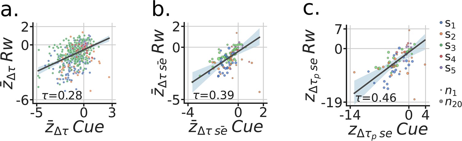
(a) Linear zone encoding model with reward , at a given sample time , the current position of the animal and the reward identity is multiplied by learned weights to predict FR for each recorded unit . (b) Example time window of , the true FR in black and the predicted FR in red . (c) Model comparison between three types of zone Encoding during inbound trajectories: , , . Each dot is a unit, blue dots were negative , red scales with and y-axis. (d) Model comparison scores. Y-axis is the Mann-Whitney Z transformed statistic for comparing the on test folds. Color-bar indicates the median difference in across test folds.
Figure 6
Modeling navigational/spatial variables in neural coding during open-field foraging.
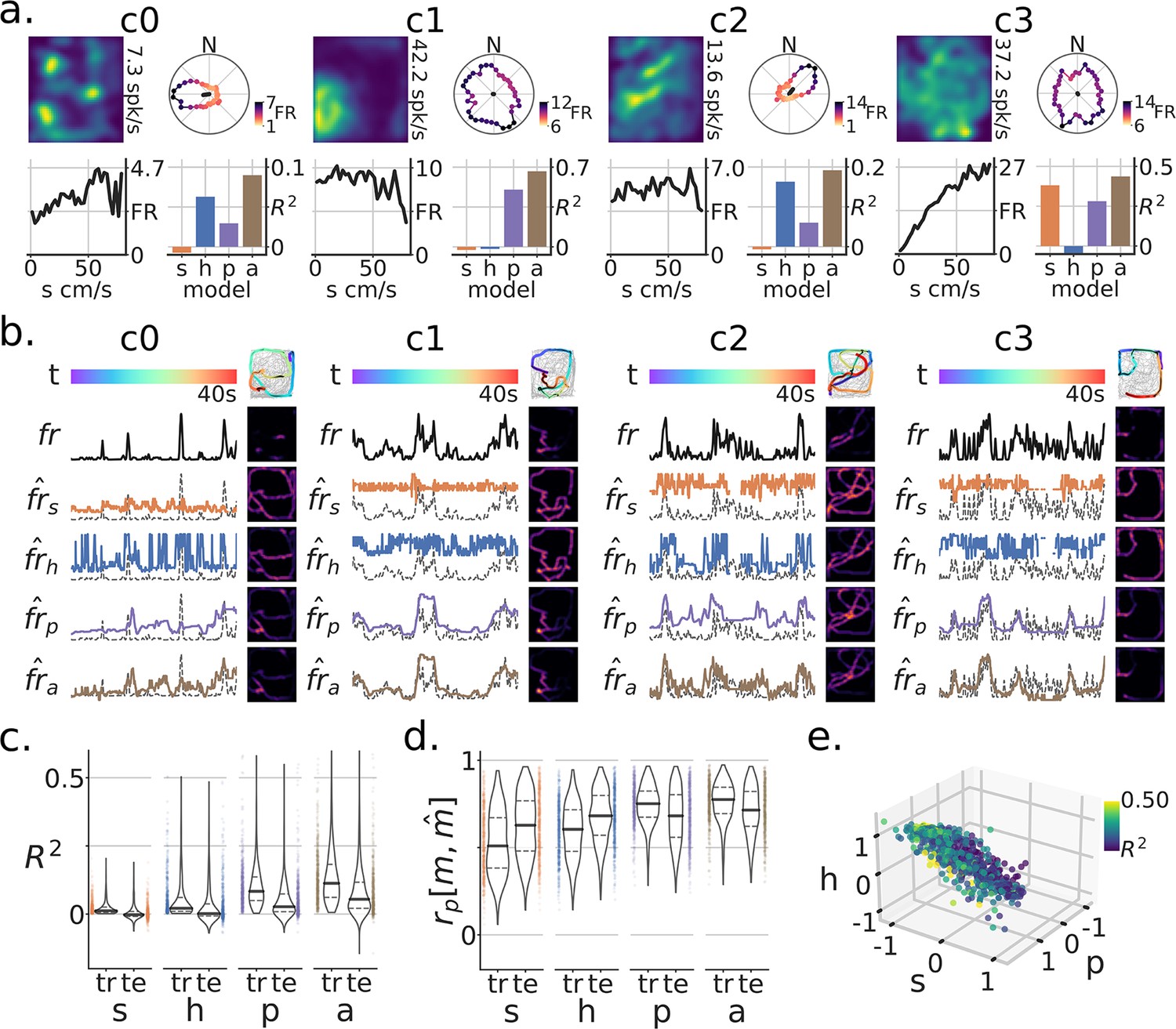
(a) Neural responses of four example units for subjects foraging an open-field (OF) arena [1.3m x 1.5m]. For each unit sub-panel (c0–c3): top-left, firing-rate map (number is the peak FR); top-right, head-direction tuning curve, color indicates FR magnitude by angle; bottom-left, speed tuning curve (s=speed); bottom-right, model-based variance explained on test data () by variable (h=heading-direction, P=position, a=aggregate model). (b) Model-based responses by variable for a selected test time-window for units c0-c3. Each row corresponds to a different model prediction (), the true firing-rate (fr) for that unit, or at the top the color-coded time-window (t). Top-right, the data on which the model was trained is in grey and super-imposed is the test-window color-coded by time and with firing rate magnitude in increasing dot-size. Other heat-maps are the resulting firing-rate maps generated for the test trajectory. Model predicted rates are shown with colors matching (a), with the background dotted line being the true (fr) (a). (c) Population level () for train (tr) and test (te) sets. (d) Population level firing-rate map Pearson correlation between true and predicted maps . Note that for both metrics, the aggregate model and the position model produced the best results. (e) Relationship between coefficients on the aggregate model by unit. The color corresponds to the model’s training set .
Figure 7 with 3 supplements
Matched units across tasks reveal that head-direction coding units remap the strongest.
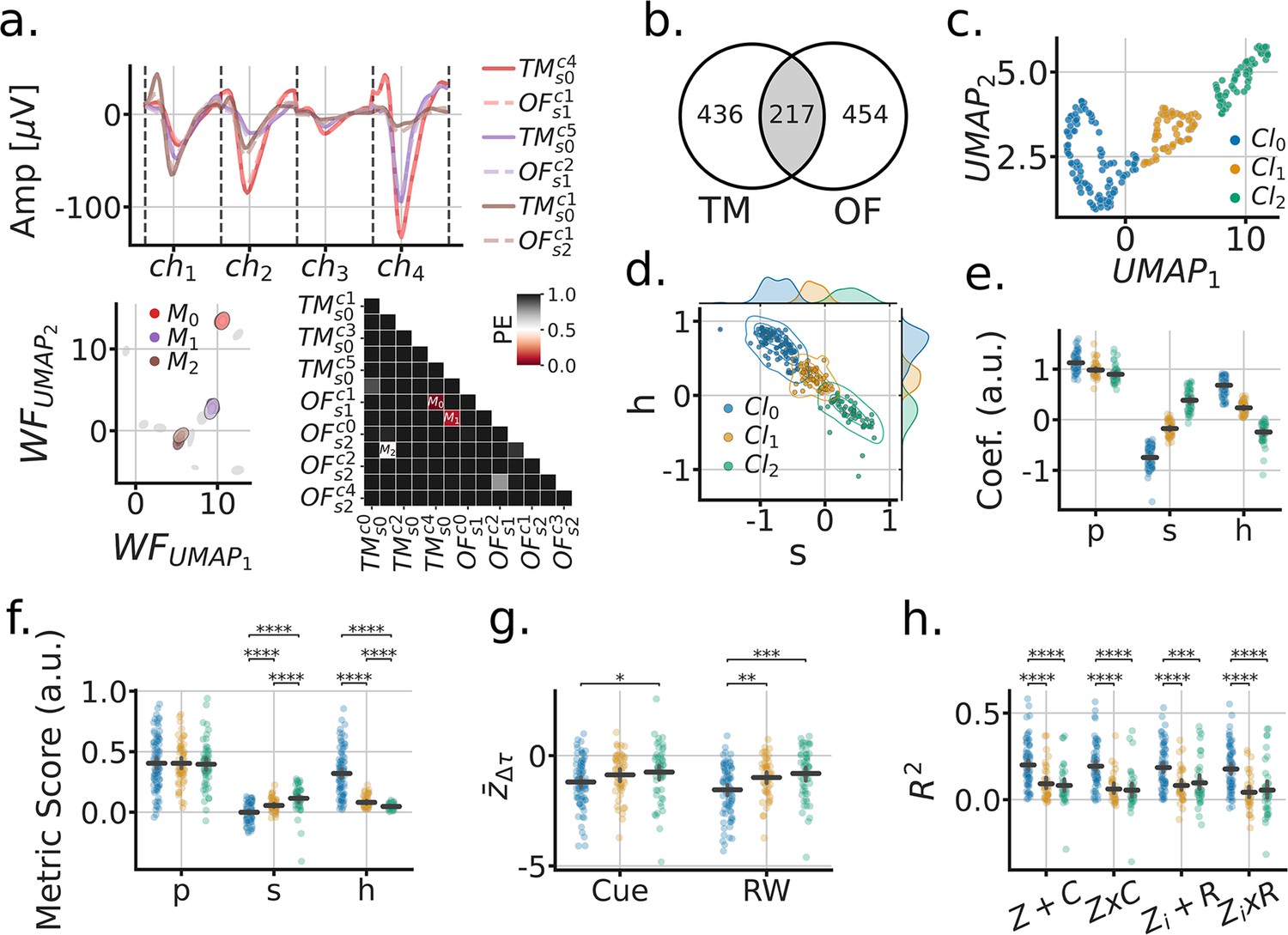
(a) Procedure for matching units across tasks (OF-open field, TM-tree maze). Top, 6 tetrode waveforms color-coded by matched units; bottom-left, fitted Gaussians to the dimensionally reduced unit waveforms for that tetrode across matched depth sessions (grey, unmatched units); bottom-right, symmetric confusion error matrix across units, threshold for matching . (b) Venn diagram of matched units across tasks. (c) UMAP clustering of the aggregate model coefficients for matched units. (d) Head-direction (h) vs speed (s) coefficients formed a clustering subspace. (e) Model coefficients of aggregate model used for finding clusters (P=position). Horizontal lines are the population mean, and error bars are the mean’s 95% CI. Statistics not performed, as the clusters were fitted from these parameters. (f) Tuning metric scores (P=split half rate-map correlation; s=speed-score; h=resultant-vector length score). Paired statistics through Mann-Whitney U tests (*= , **= , ***= , ****= ) (g) Remap scores by OF cluster. (h) TM model scores by OF cluster.
Figure 7—figure supplement 1
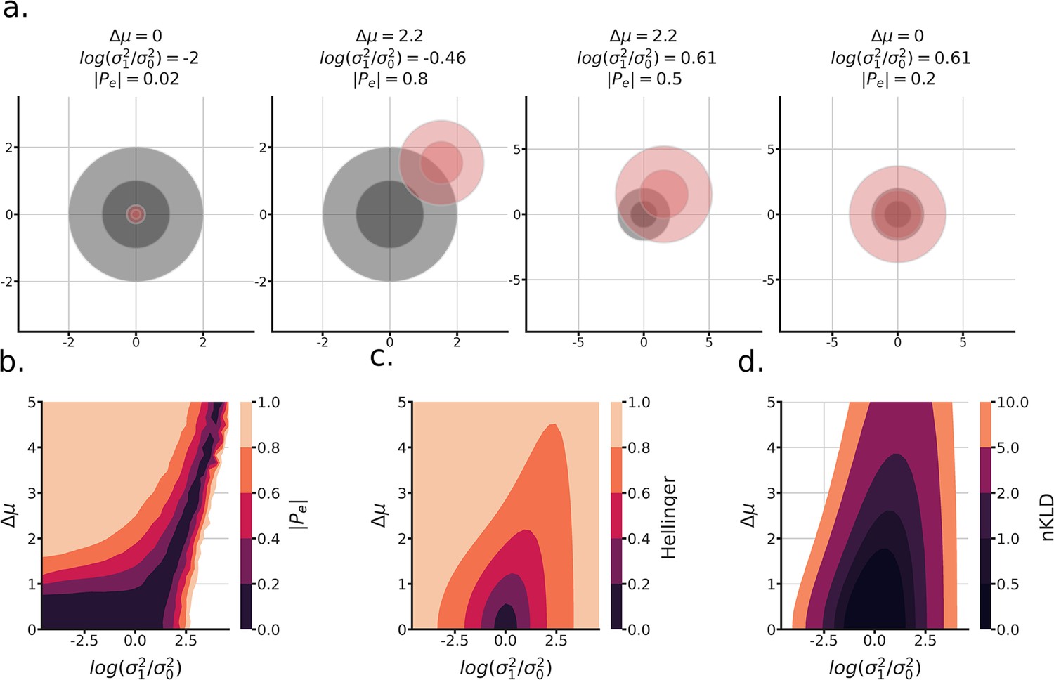
Demonstration of waveform matching algorithm.
This algorithm was followed to determine which units were recorded in both the open-field and Tree-Maze tasks. We operationalized this matching by quantifying how likely it is that given the waveform of random spike it would be incorrectly assigned to the correct cluster. (a) Four simulated scenarios of the resulting wave clusters for two units, parameterized by their difference in location , and their log-ratio of variances . The metric is also shown for each example, this represents the probability of mistaking a waveform for the other. If this value is less than 0.5, we say that given the data, those units are not distinguishable from another and are thus matched. In these examples, only the second from the left would not be matched . Note that while asymmetry is possible, (e.g. of to is different than of to ), that scenario was not of interest for our study and values are averaged for each pair. (b) Full landscape of for the parametrization between a pair of units. Note that there is a band of matching along this landscape. (c-d) Hellinger and normalized KLD distances. Note that these metrics tend to reflect the ‘closeness’ of the mean/variance of the distributions, which is not the main goal of the matching algorithm.
Figure 7—figure supplement 2
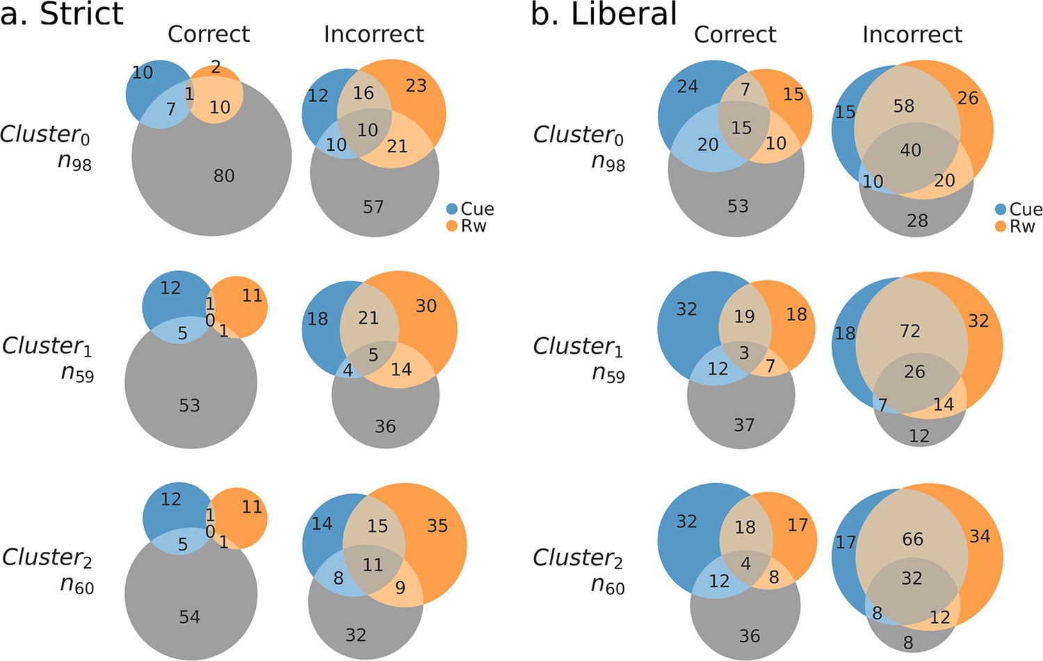
Cue and reward rate coding vs correct/incorrect interaction and cluster identity.
These analyses use the functionally defined clusters of units identified in the open-field arena. Thresholds for correct/incorrect as described in Figure 4—figure supplement 6. (a) Strict correct/incorrect coding. (b). Liberal correct/incorrect coding, groupings in (a). are part of (b). There is little overlap between the open-field clusters and correct coding for both cue and reward, while the overlap is larger for incorrect coding. At the same time, most incorrect coding units did not fall into any of the clusters, suggesting that the Tree-Maze task recruits a different population of neurons that are either inactive or were not detected in the Open-Field task.
Figure 7—figure supplement 3
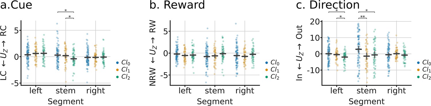
Differences in activity rates by cluster and condition.
These analyses use the functionally defined clusters of units identified in the open-field arena. (a) Outbound cue firing rate activity difference (Mann-Whitney statistic ) between Right-Cue and Left cue by segment and cluster. (b) Inbound differences between rewarded (RW) and not-rewarded (NRW) trials. (c) Differences in representation for Outbound (Out) and Inbound (In) trajectories. Note the higher variability for cluster 0, consistent with that cluster containing Head-Direction units.
Additional files
Download links
A two-part list of links to download the article, or parts of the article, in various formats.
Downloads (link to download the article as PDF)
Open citations (links to open the citations from this article in various online reference manager services)
Cite this article (links to download the citations from this article in formats compatible with various reference manager tools)
Parahippocampal neurons encode task-relevant information for goal-directed navigation
eLife 12:RP85646.
https://doi.org/10.7554/eLife.85646.3


