Social learning mechanisms shape transmission pathways through replicate local social networks of wild birds
- Edward Grey Institute of Field Ornithology, Department of Biology, University of Oxford, United Kingdom
Figures
Figure 1 with 4 supplements

Schematic overview of the simulation procedure.
First, a weekly social network of one of the feeder locations (shown as black dots) in the study site was selected. Second, behavioural spread was simulated on the selected network using four different social learning rules (i.e. simple, threshold, proportion, and conformity). The starting point (i.e. the first individual performing the new behaviour) was randomly chosen. Then, at each timestep (t1–tn), a naive individual adopted the novel behaviour with a given probability of the adoption event being from social learning (dependent on the social learning rule at play; see methods for further details) until all individuals in the network had adopted the novel behaviour. Third, we calculated a correlation coefficient (Spearman’s rank correlation coefficient) between three individual social network metrics (i.e. weighted clustering coefficient, weighted degree, and weighted betweenness) and the order (i.e. timestep) in which individuals adopted the novel behaviour. Finally, we repeated this process 100 times for each weekly, local social network.
Figure 1—figure supplement 1
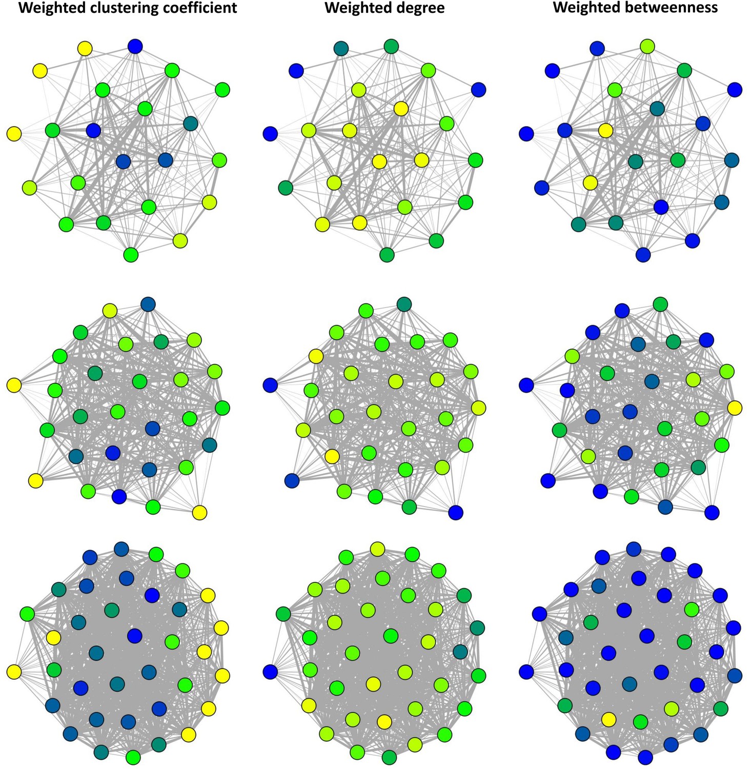
Great tit social networks illustrating individuals’ different social network positions.
Each row shows one weekly, local network of different size (top to bottom: 22, 29, 39 individuals). Columns show the three social network metrics (weighted clustering coefficient, weighted degree, and weighted betweenness) and colours represent the range in network metrics (yellow indicates larger values and blue smaller values).
Figure 1—figure supplement 2
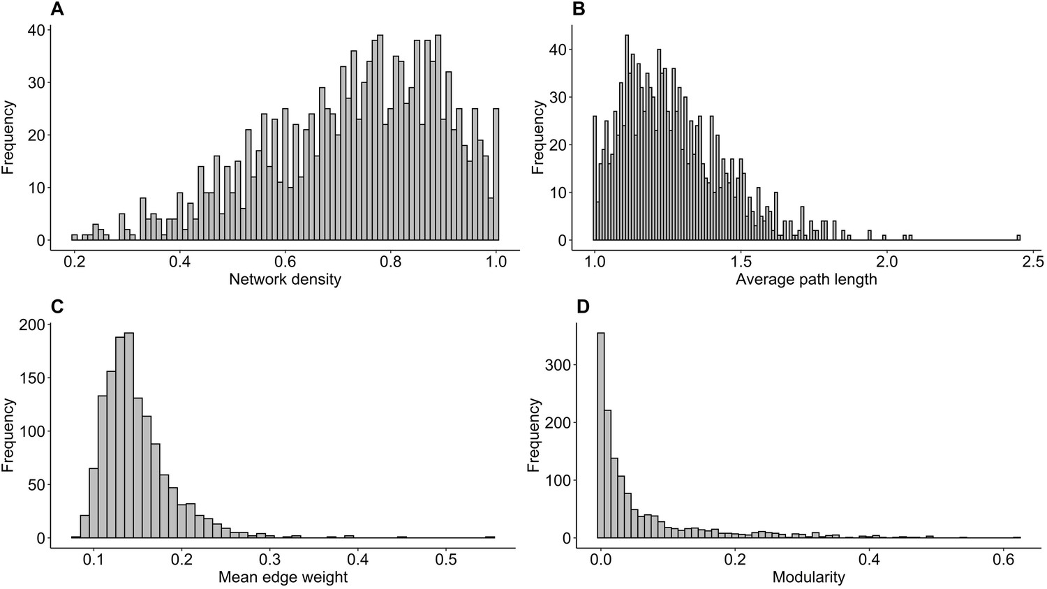
Data distribution of four global network metrics from the 1343 weekly, local social networks.
(A) Network density, calculated as the number of existing connections divided by all potential connections. (B) Average path length. (C) Mean edge weight defined as the average of all edge weights in a network (excluding zero edges). (D) Modularity, inferred as the structural communities (modularity index Q) for each network using the edge betweenness community detection algorithm. We calculated the four global network metrics using the package ‘igraph’ (Csardi and Nepusz, 2006). The network density was calculated as the number of existing connections divided by all potential connections. The global clustering coefficient was defined as the ratio of the triangles and the connected triples within the network. We inferred the structural communities (modularity index Q) for each network using the edge betweenness community detection algorithm. The average edge strength was defined as the average of all edge weights in a network (excluding zero edges).
Figure 1—figure supplement 3
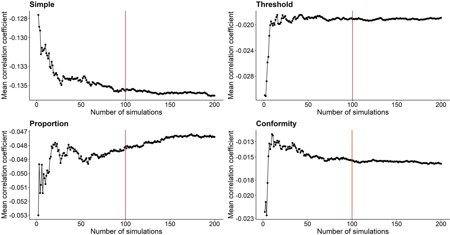
Mean correlation coefficient between weighted degree and order of acquisition in relation to different numbers of simulations.
After about 100 simulation runs (red vertical line), mean correlation coefficients do not fluctuate anymore to a large extent. Therefore, 100 simulation runs were chosen as a meaningful cut-off.
Figure 1—figure supplement 4
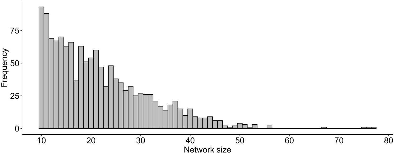
Data distribution of network sizes (i.e. the number of individuals each network contained).
Figure 2 with 5 supplements
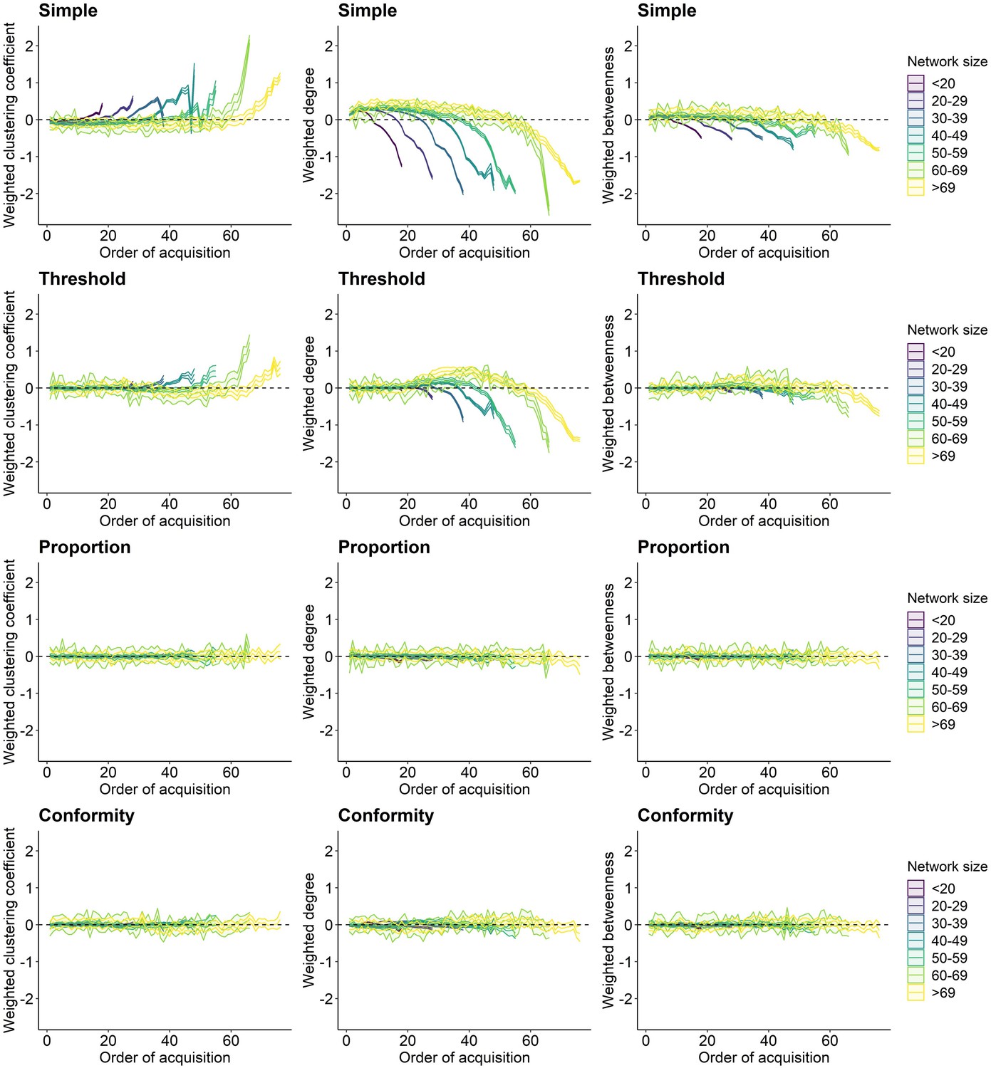
Relationship between individual network metric and the order of acquisition for each social learning rule.
Each column shows a different network metric (left to right: weighted clustering coefficient, weighted degree, and weighted betweenness). Each row represents one of the four spreading rules (top to bottom: simple, threshold, proportion, and conformity). Lines plot the average network metric for each order of acquisition and ribbons show the 95% confidence interval from the 100 simulations for each binned group of network sizes. Colour represents network size with darker colour indicating smaller networks. The social transmission rate, the threshold location, and the frequency dependence parameter were set to 5.
Figure 2—figure supplement 1
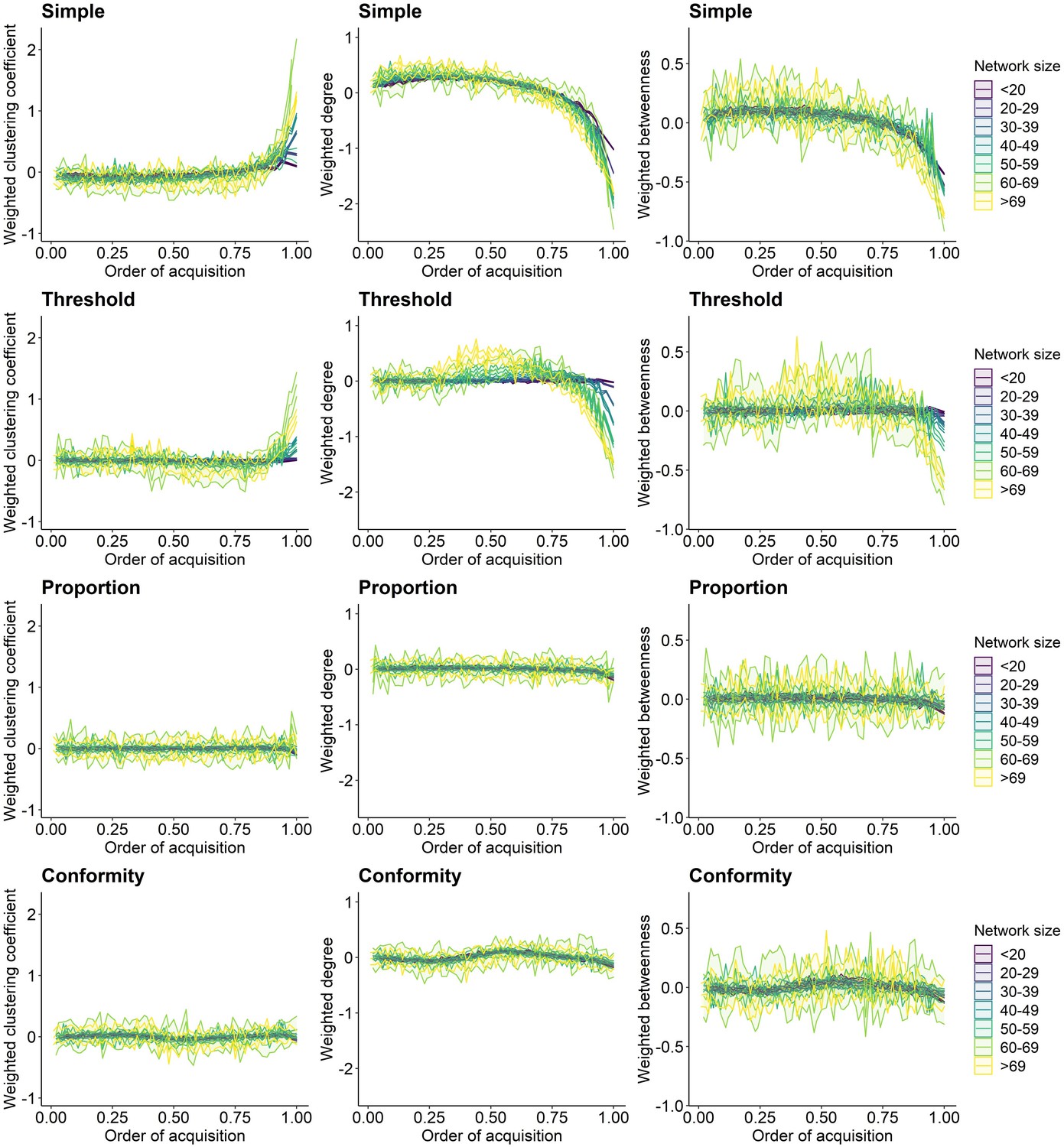
Relationship between individual network metric and the standardized order of acquisition (OAC) for each transmission rule and split by network size.
Each column shows a different network metric (left to right: weighted clustering coefficient, weighted degree, and weighted betweenness). Each row represents one of the four spreading rules (top to bottom: simple, threshold, proportion, and conformity). A value of OAC = 0.5 corresponds to 50% of individuals within the social network being knowledgeable. Lines show the average network metric for each OAC and ribbons show the 95% confidence interval from the 100 simulations for each binned group of network sizes. Colour represents network size with darker colour indicating smaller sizes. The social transmission rate ‘s’, the threshold location ‘a’, and the frequency dependence ‘f’ were set to 5.
Figure 2—figure supplement 2
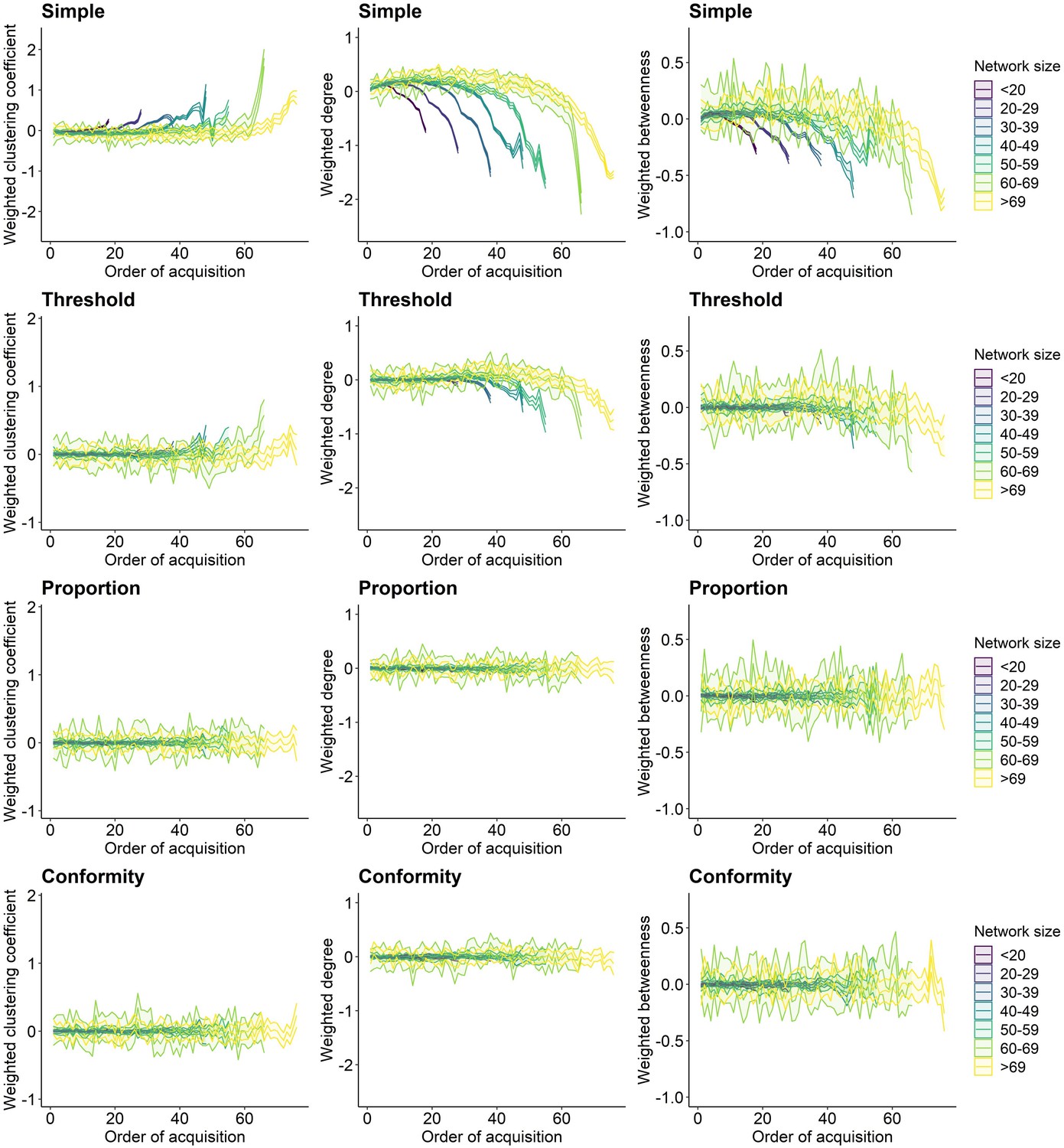
Relationship between individual network metric and the order of acquisition for each social learning rule with a social learning rate of 1.
Each column shows a different network metric (left to right: weighted clustering coefficient, weighted degree, and weighted betweenness). Each row represents one of the four spreading rules (top to bottom: simple, threshold, proportion, and conformity). Lines plot the average network metric for each order of acquisition and ribbons show the 95% confidence interval from the 100 simulations for each binned group of and network sizes. Colour represents network size with darker colour indicating smaller networks. The threshold location ‘a’ and the frequency dependence ‘f’ were set to 5.
Figure 2—figure supplement 3
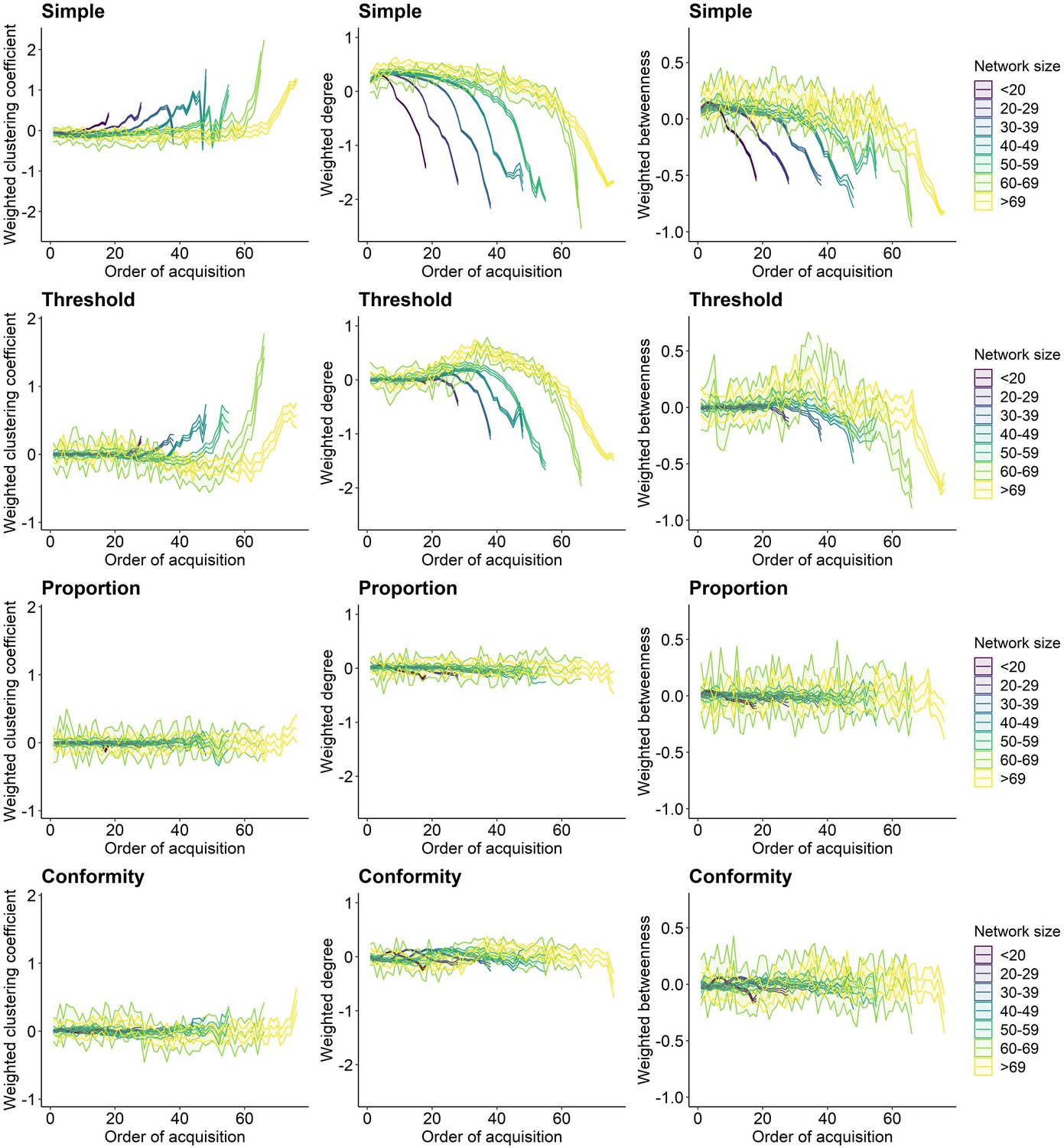
Relationship between individual network metric and the order of acquisition for each social learning rule with a social learning rate of 10.
Each column shows a different network metric (left to right: weighted clustering coefficient, weighted degree and weighted betweenness). Each row represents one of the four spreading rules (top to bottom: simple, threshold, proportion, and conformity). Lines plot the average network metric for each order of acquisition and ribbons show the 95% confidence interval from the 100 simulations for each binned group of and network sizes. Colour represents network size with darker colour indicating smaller networks. The threshold location ‘a’ and the frequency dependence ‘f’ were set to 5.
Figure 2—figure supplement 4
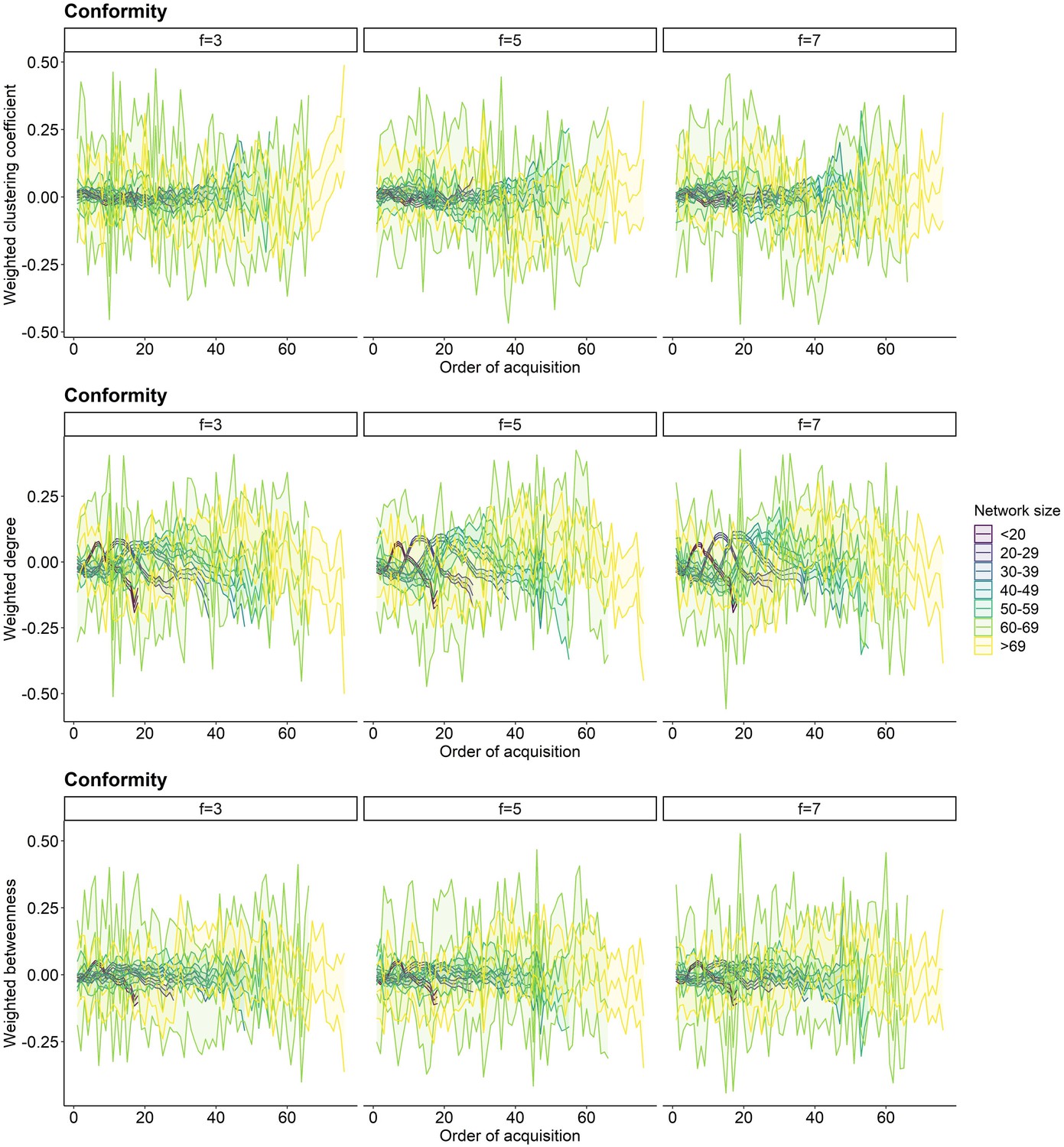
Relationship between individual network metric and the order of acquisition for the conformity learning rule under different frequency-dependent values ‘f’.
Each row shows a different network metric (top to bottom: weighted clustering coefficient, weighted degree, and weighted betweenness). Each column represents a different parameter for the frequency dependence variable ‘f’. Lines plot the average network metric for each order of acquisition and ribbons show the 95% confidence interval from the 100 simulations for each binned group of network sizes. Colour represents network size with darker colour indicating smaller networks. The social transmission rate was set to 5.
Figure 2—figure supplement 5
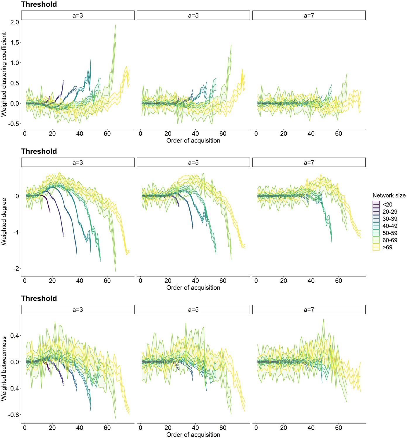
Relationship between individual network metric and the order of acquisition for the threshold learning rule under different threshold locations ‘a’.
Each row shows a different network metric (top to bottom: weighted clustering coefficient, weighted degree, and weighted betweenness). Each column represents a different parameter for the threshold location ‘a’ (3–7). Lines plot the average network metric for each order of acquisition and ribbons show the 95% confidence interval from the 100 simulations for each binned group of network sizes. Colour represents network size with darker colour indicating smaller networks. The social transmission rate was set to 5.
Figure 3 with 2 supplements
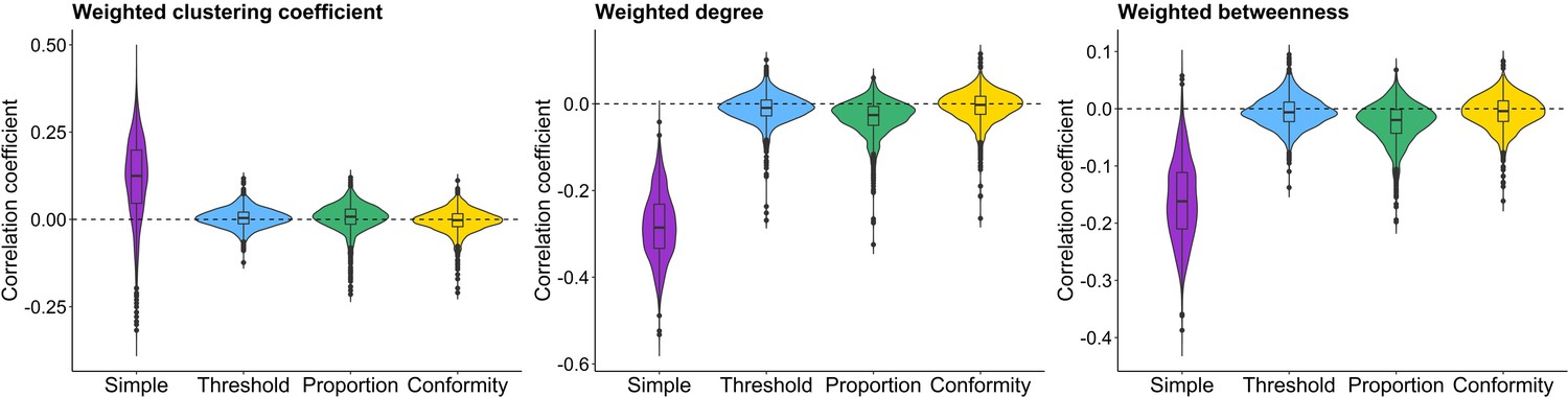
Distribution of average correlation coefficients for each social learning rule and network metric.
Violin and boxplots show the distribution of the average correlation coefficients between individual network metric and order of acquisition across 100 simulations from each network for each of the four social learning rules (i.e. simple, proportion, conformity, and threshold). Each plot shows one of the individual network metrics (weighted clustering coefficient, weighted degree, and weighted betweenness).
Figure 3—figure supplement 1
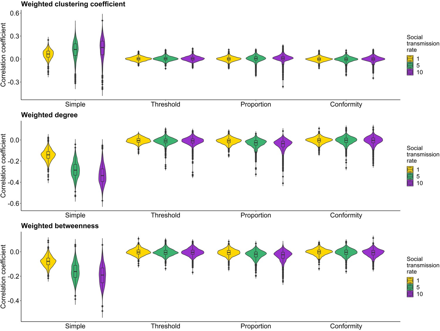
Distribution of average correlation coefficients for each social learning rule and network metric under different social learning rates.
Violin and boxplots show the distribution of the average correlation coefficients across 100 simulations from each network for each of the four social learning rules (i.e. simple, proportion, conformity, and threshold). Each plot shows one of the individual network metrics (weighted clustering coefficient, weighted degree, and weighted betweenness). Colour represents the parameter set for the social transmission rate.
Figure 3—figure supplement 2
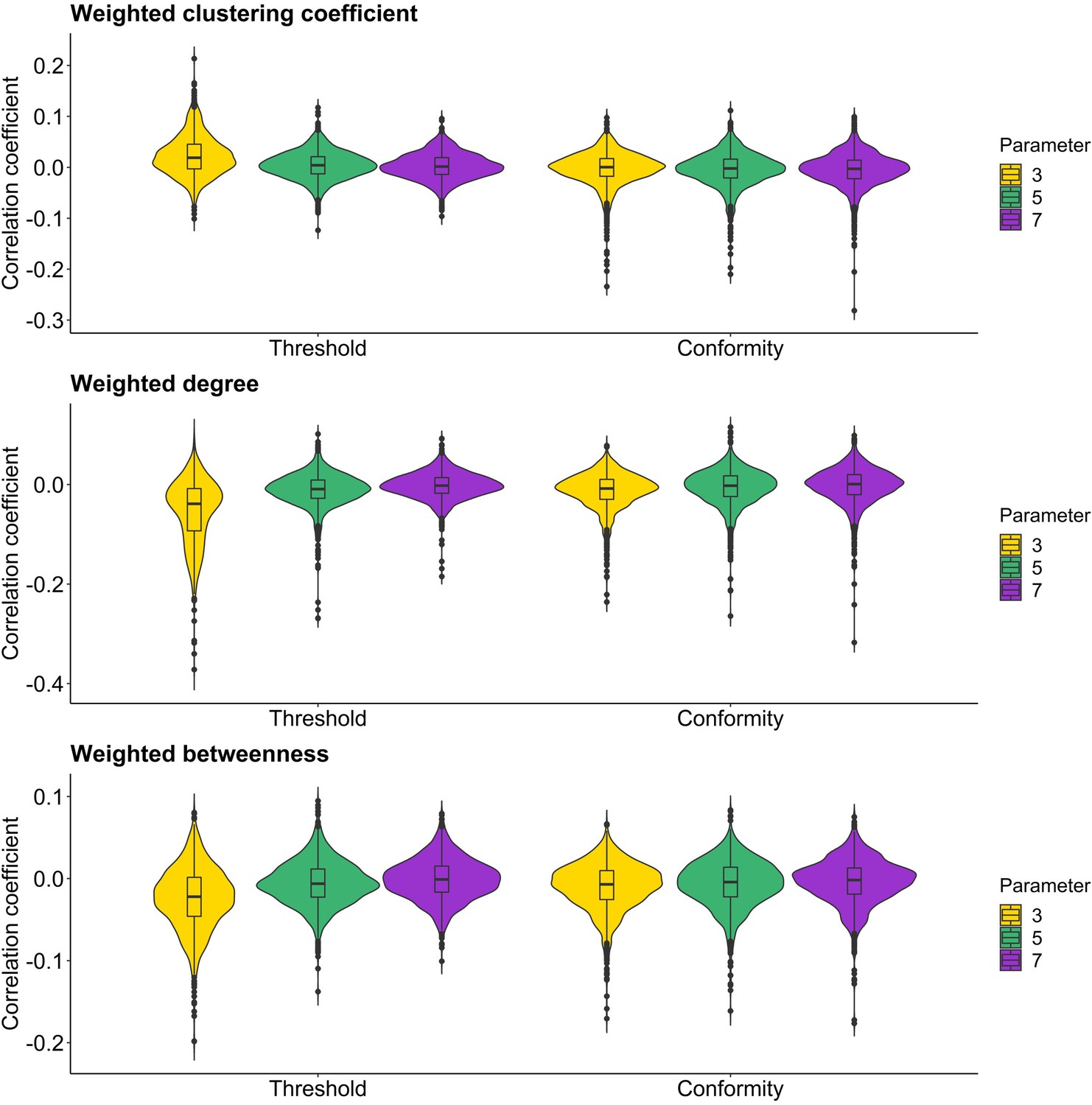
Distribution of average correlation coefficients for the threshold and conformity learning rule under different parameters.
Violin and boxplots show the distribution of the average correlation coefficients across 100 simulations from each network for each of the four social learning rules (i.e. simple, proportion, conformity, and threshold). Each plot shows one of the individual network metrics (weighted clustering coefficient, weighted degree, and weighted betweenness). Colour represents the parameter set for the social transmission rate.
Figure 4 with 2 supplements
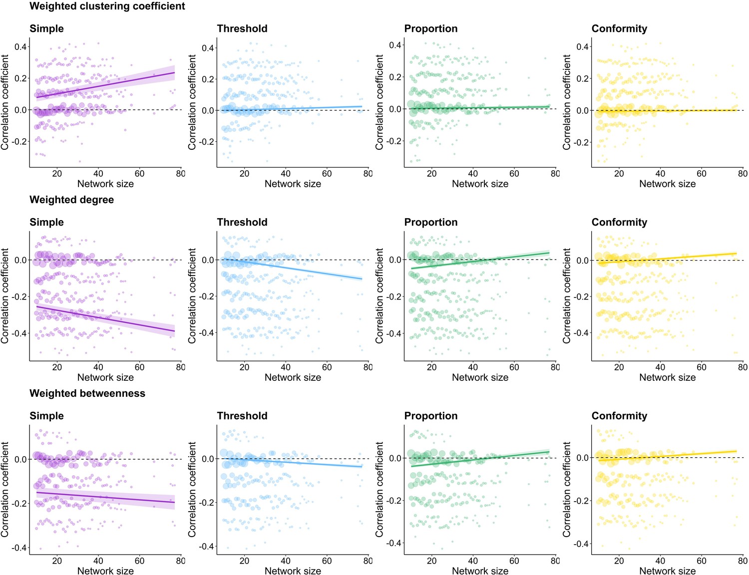
Relationship between correlation coefficient and network size across the four social learning rules.
Each row shows one of the individual network metrics (top to bottom: weighted clustering coefficient, weighted degree, and weighted betweenness) and each column a different social learning rule (left to right: simple, threshold, proportion, and conformity). Average correlation coefficients across the 100 simulations per network are plotted as count dots (larger dots indicate more values for the respective value), lines represent the predicted effects generated from linear mixed-effect models (LMM) and ribbons represent the 95% confidence intervals (see Supplementary file 1b for model results).
Figure 4—figure supplement 1
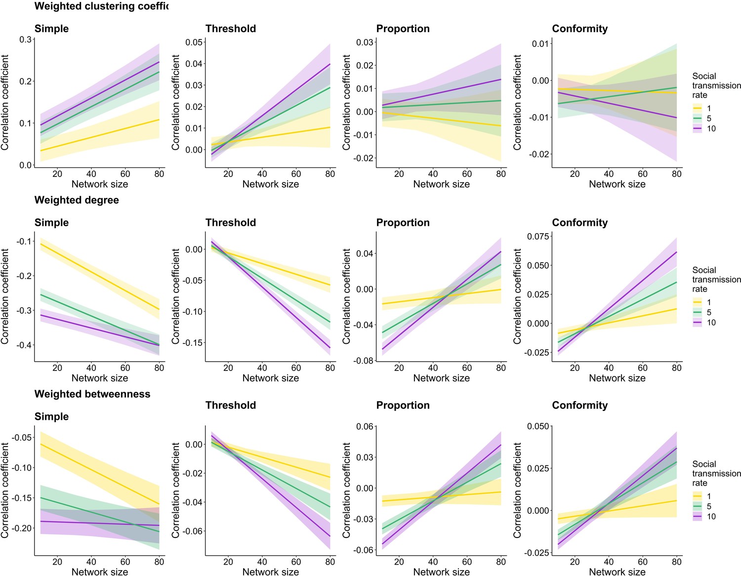
Relationship between correlation coefficient and network size across the four social learning rules under different social learning rates.
Each row shows one of the individual network metrics (top to bottom: weighted clustering coefficient, weighted degree, and weighted betweenness) and each column a different social learning rule (left to right: simple, threshold, proportion, and conformity). Lines show the predicted effects generated from linear mixed-effect models (LMM) and ribbons show the 95% confidence intervals (see Supplementary file 1b for model results). Colour represents the different parameters set for the social transmission rate.
Figure 4—figure supplement 2
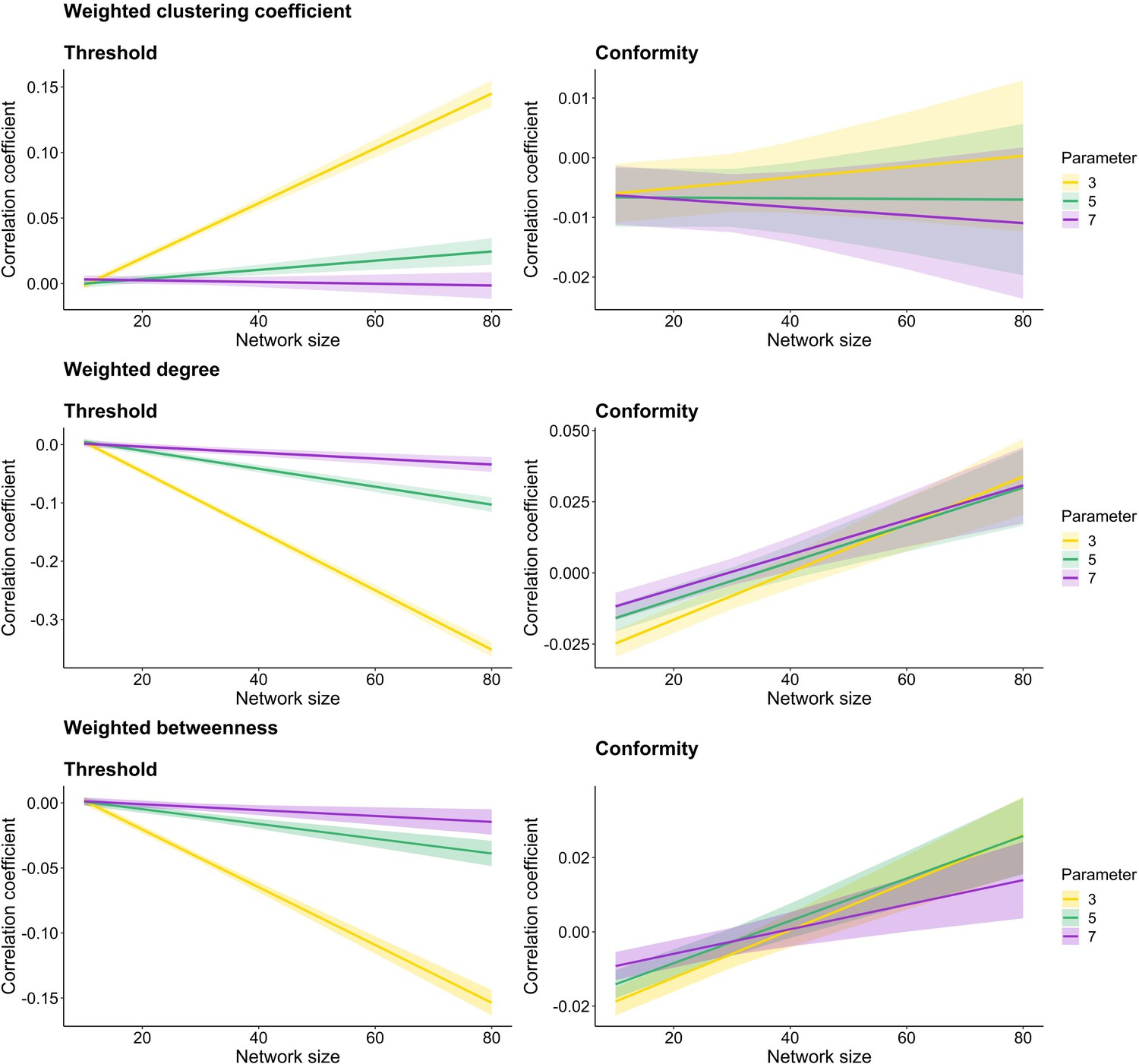
Relationship between correlation coefficient and network size for the threshold and conformity learning rule under different parameters.
Each row shows one of the individual network metrics (top to bottom: weighted clustering coefficient, weighted degree, and weighted betweenness) and each column a different social learning rule (left to right: simple, threshold, proportion, and conformity). Lines show the predicted effects generated from linear mixed-effect models (LMM) and ribbons show the 95% confidence intervals (see Supplementary file 1b for model results). Colour represents the different parameters set for the social transmission rate.
Figure 5 with 2 supplements
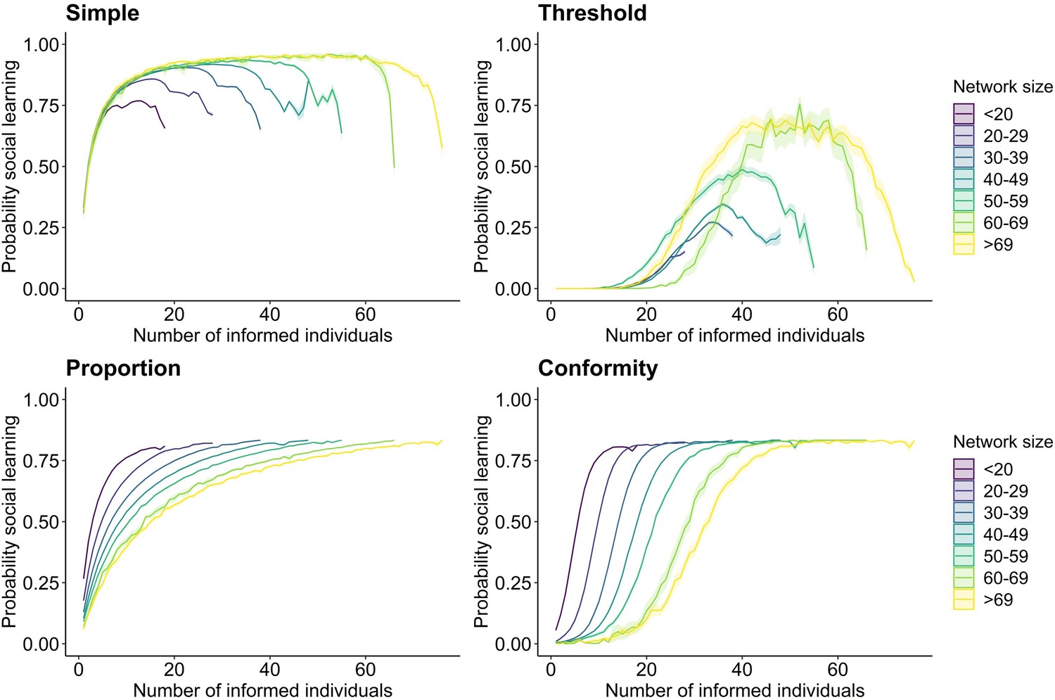
Relationship between the probability of an individual socially adopting the seeded behaviour and the number of informed individuals within the network.
Panels show the results for each of the four social learning rules (simple, threshold, proportion, and conformity). The x-axis describes the number of informed individuals within a social network. The simulations are set so that at each timestep a new individual adopts the behaviour, whereby each time each individual has a probability of adopting the behaviour through social learning (y-axis) given the set learning rule. Lines plot the average probability for each timestep and ribbons show the 95% confidence intervals from the 100 simulations across the binned groups for different network sizes. Colour represents network size with darker colour indicating smaller networks. The social transmission rate, the threshold location, and the frequency dependence parameter were set to 5.
Figure 5—figure supplement 1
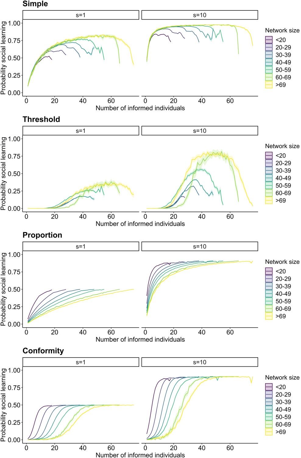
Relationship between the probability of an individual socially adopting the seeded behaviour and the number of informed individuals within the network under different social transmission rates.
Columns show the results for two different social transmission rates (s = 1, s = 10, see main text for results on s = 5). Rows show results for the four social learning rules (simple, threshold, proportion, and conformity). The x-axis describes the number of informed individuals within a social network. At each timestep a new individual adopted the seeded behaviour, whereby each time each individual has a probability of adopting the behaviour through social learning (y-axis) given the set learning rule. Lines plot the average probability for each timestep and ribbons show the 95% confidence intervals from the 100 simulations across the binned groups for different network sizes. Colour represents network size with darker colour indicating smaller networks.
Figure 5—figure supplement 2
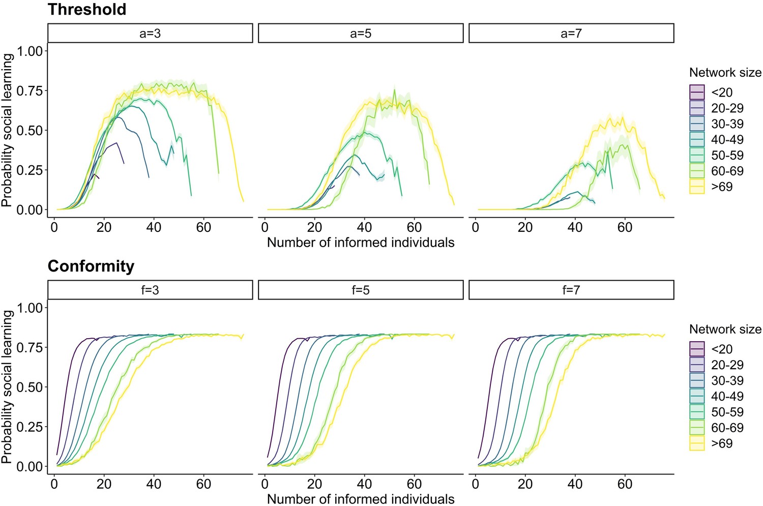
Relationship between the probability of an individual socially adopting the seeded behaviour and the number of informed individuals within the network under different threshold location (a) and frequency dependence (f) parameters.
Plots on the top show results for the threshold model, plots on the bottom results for the conformity model. Columns show for each model different parameters, that is threshold location (a) and frequency dependence (f) parameters (left to right: 3, 5, 7). At each timestep a new individual adopted the seeded behaviour, whereby each time each individual has a probability of adopting the behaviour through social learning (y-axis) given the set learning rule. Lines plot the average probability for each timestep and ribbons show the 95% confidence intervals from the 100 simulations across the binned groups for different network sizes. Colour represents network size with darker colour indicating smaller networks.
Author response image 1
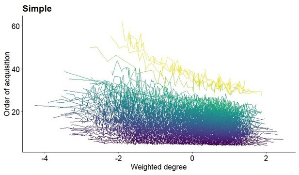
Relationship between order of acquisition and weighted degree for the simple learning rule.
Lines plot the average OAC for each value of weighted degree (scaled) and network size from the 100 simulations of each network. Colour represents network size with darker colour indicating smaller networks.
Additional files
-
Supplementary file 1
Supplementary tables.
(a) Correlation coefficients between the three individual network metrics. Shown are the correlation coefficient between the network metrics weighted clustering coefficient, degree, and betweenness. (b) Effects of network size on the mean correlation coefficient. Shown are the effects of network size on the mean correlation coefficient for weighted clustering coefficient, degree, and betweenness for each of the four social learning models. We report the estimate, the standard error (SE), test statistic (t), and p values.
- https://cdn.elifesciences.org/articles/85703/elife-85703-supp1-v1.docx
-
MDAR checklist
- https://cdn.elifesciences.org/articles/85703/elife-85703-mdarchecklist1-v1.docx
Download links
A two-part list of links to download the article, or parts of the article, in various formats.
Downloads (link to download the article as PDF)
Open citations (links to open the citations from this article in various online reference manager services)
Cite this article (links to download the citations from this article in formats compatible with various reference manager tools)
Social learning mechanisms shape transmission pathways through replicate local social networks of wild birds
eLife 12:e85703.
https://doi.org/10.7554/eLife.85703


