Temperature sensitivity of the interspecific interaction strength of coastal marine fish communities
- Hakubi Center, Kyoto University, Japan
- Center for Ecological Research, Kyoto University, Japan
- Department of Ocean Science, The Hong Kong University of Science and Technology, Clear Water Bay, China
- Natural History Museum and Institute, Japan
- Maizuru Fisheries Research Station, Kyoto University, Japan
- Fisheries Technology Institute, Japan Fisheries Research and Education Agency, Japan
- Graduate School of Life Sciences, Tohoku University, Japan
Figures
Figure 1 with 2 supplements
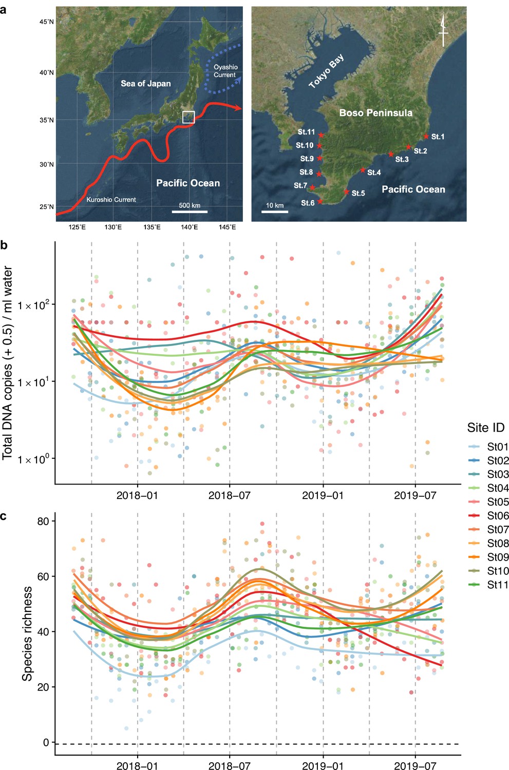
Study sites and overall dynamics of environmental DNA (eDNA) concentrations and the number of fish species detected.
(a) Study sites in the Boso Peninsula. The study sites are influenced by the Kuroshio Current (red arrow; left panel) and distributed along the coastal line in the Boso Peninsula (right panel). (b) Total eDNA copy numbers estimated by quantitative eDNA metabarcoding (see Methods for detail). (c) Fish species richness detected by eDNA metabarcoding. Points and lines indicate raw values and LOESS lines, respectively. The line color indicates the sampling site. Warmer colors generally correspond to study sites with a higher mean water temperature.
Figure 1—figure supplement 1
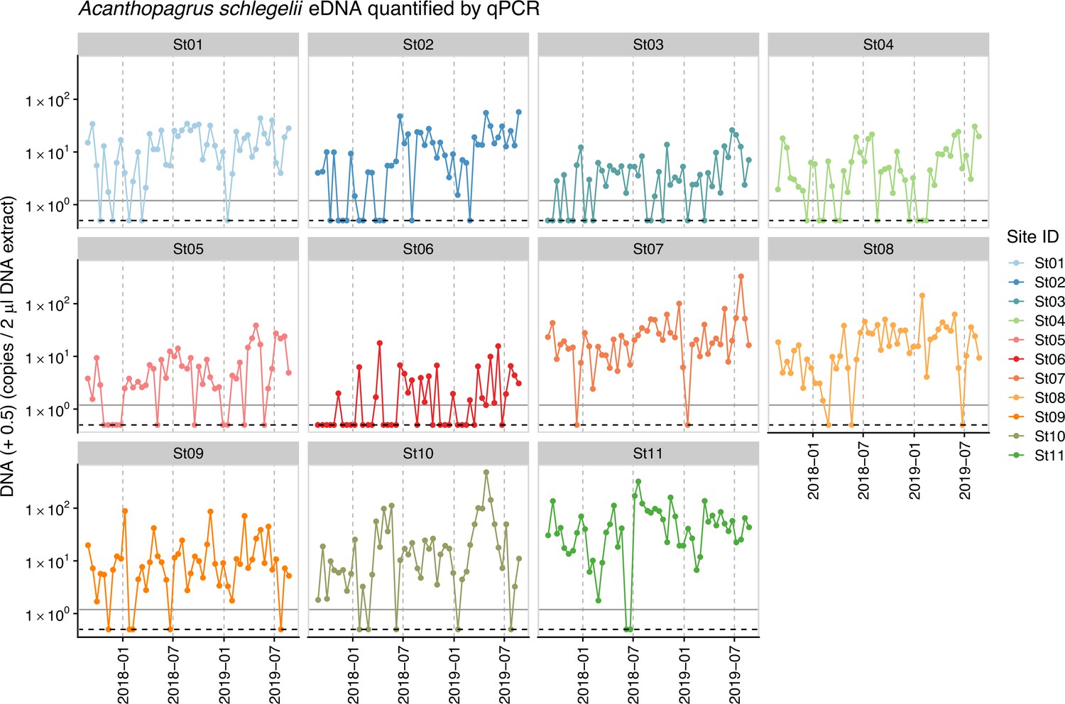
Dynamics of environmental DNA (eDNA) copy numbers of Japanese black seabream (Acanthopagrus schlegelii) that was used as an internal standard.
Gray horizontal line indicates the minimum eDNA copy number of Japanese black seabream detected. Approximately 83.3% of samples contain detectable concentrations of the standard DNA, which was used to convert sequence reads to eDNA copy numbers. For samples which do not contain the standard DNA, we assume that it contains the minimum amount of eDNA copy numbers (i.e., 0.69 copies/2 extracted DNA; gray horizontal line).
Figure 1—figure supplement 2
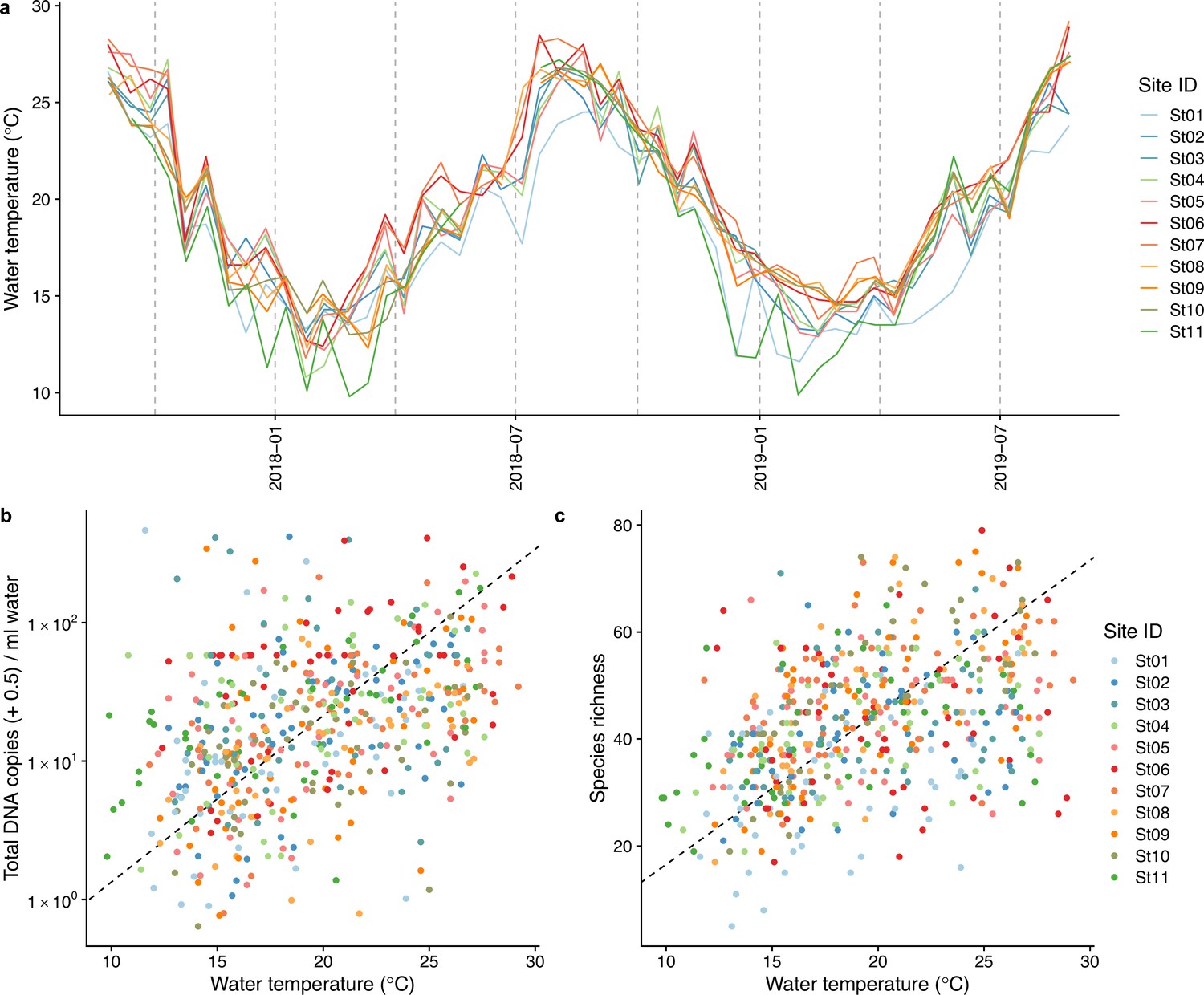
Dynamics of water temperature and the relationships between water temperature and total environmental DNA (eDNA) concentration and fish species richness.
(a) Dynamics of sea surface water temperature at the sampling sites. (b) The relationship between water temperature and total eDNA copy numbers, and (c) the relationship between water temperature and fish species richness. Colors indicate sampling sites. For (b) and (c), dashed lines indicate standardized major axis regression.
Figure 2 with 1 supplement
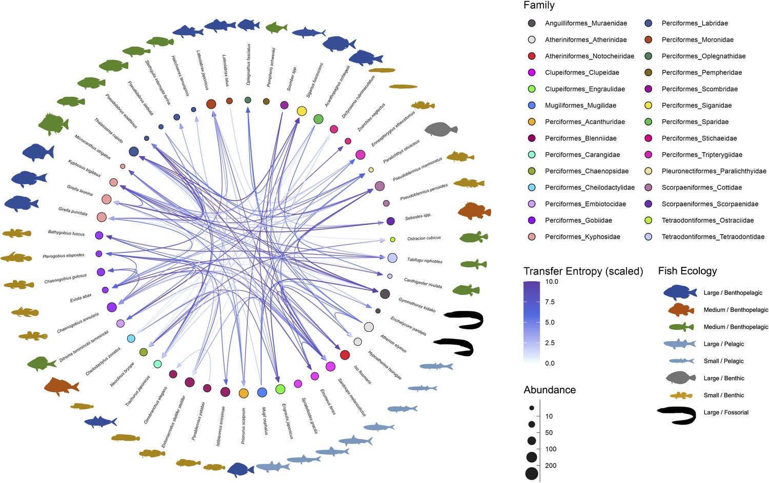
Interaction networks of the fish community in the Boso Peninsula coastal region.
The ‘average’ interaction network reconstructed by quantifying information transfer between environmental DNA (eDNA) time series. Transfer entropy (TE) was quantified by leveraging all eDNA time series from multiple study sites to draw this network. Only information flow larger than 80% quantiles (i.e., strong interaction) was shown as interspecific interactions for visualization. The edge color indicates scaled TE values, and fish illustration colors represent their ecology (e.g., habitat and feeding behavior). Node colors and node sizes indicate the fish family and fish abundance (total eDNA copy numbers of the fish species), respectively.
Figure 2—figure supplement 1
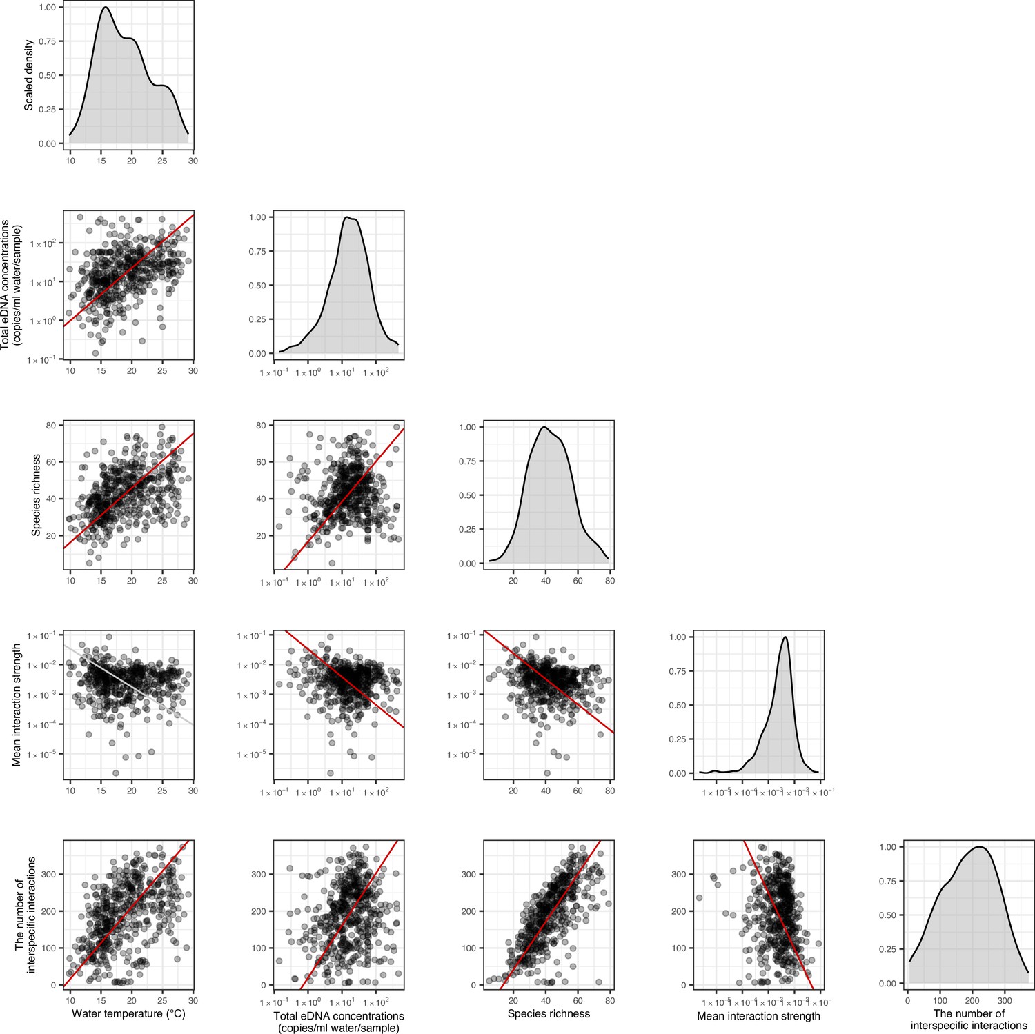
The relationships between network properties and environmental variables.
Diagonal panels show density distributions of the data, and lower triangle area shows scattered plots. Each point represents one water sample at each study site, meaning that ‘Mean interaction strength’ is a mean value at the community level. Solid red and gray lines indicate statistically clear (p < 0.05) and unclear (p > 0.05) standardized major axis regression, respectively.
Figure 3 with 3 supplements
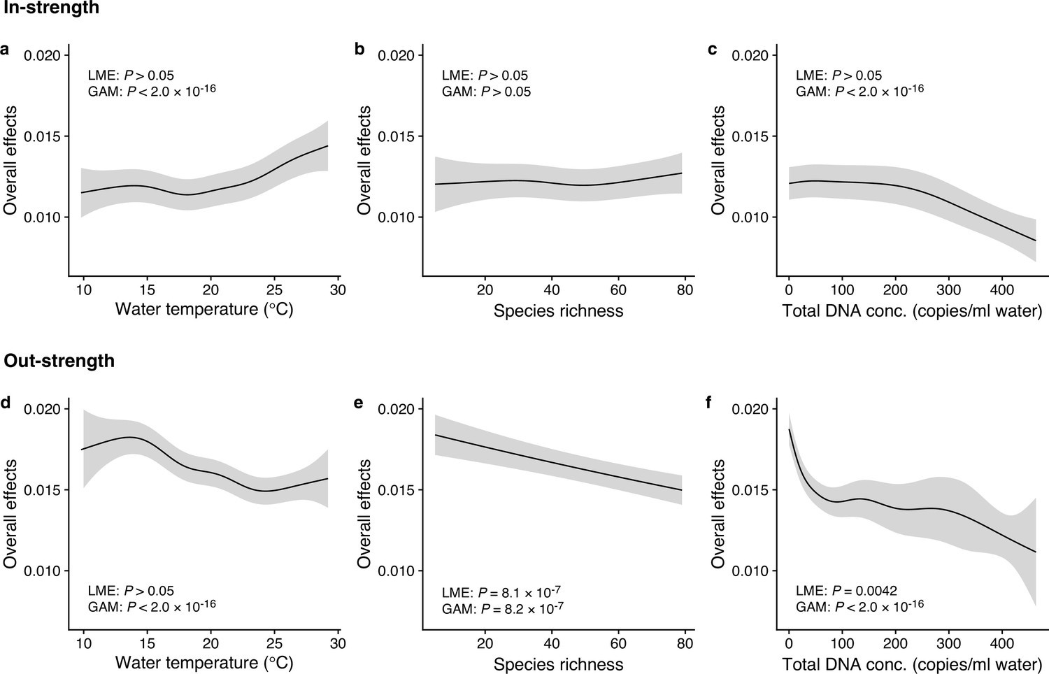
Dependence of interaction strengths on biotic and abiotic variables (50 dominant fish species and 11 study sites were leveraged).
The panels show the overall effects of biotic and abiotic variables on interaction strengths of the 50 dominant fish species: Effects of (a, d) water temperature, (b, e) species richness, and (c, f) total environmental DNA (eDNA) copy numbers. The y-axis indicates the effects of the variables on fish–fish interaction strengths quantified by the MDR S-map method. (a–c) show the effects on the species interactions that a focal species receives (i.e., in-strength), and (d–f) show the effects on the species interactions that a focal species gives (i.e., out-strength). The line indicates the average effects estimated by the general additive model (GAM), and the gray region indicates 95% confidential intervals. LME and GAM indicate the statistical clarity of the linear mixed model portion and GAM portion, respectively. Detailed statistical results and raw data are shown in Supplementary file 1d and Figure 3—figure supplement 1, respectively.
Figure 3—figure supplement 1
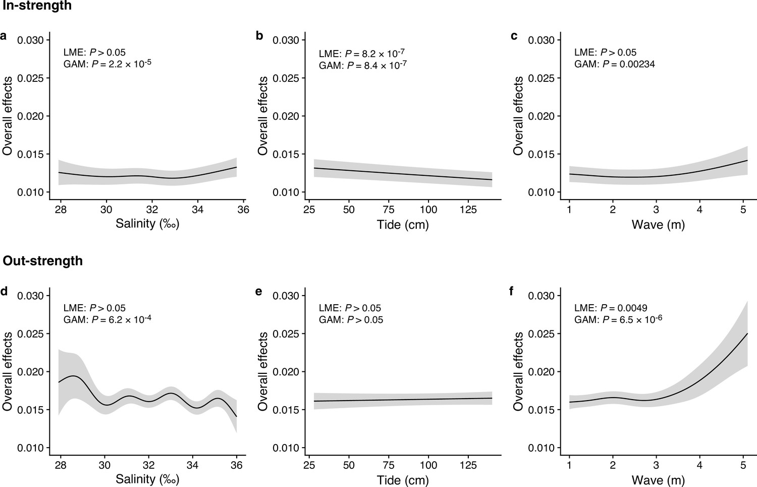
Dependence of interaction strengths on additional abiotic variables.
The panels show the overall effects of additional abiotic variables on interaction strengths of the 50 dominant fish species: Effects of (a, d) salinity, (b, e) tide level (cm), and (c, f) wave (m). The y-axis indicates the effects of environmental variables on fish–fish interaction strengths quantified by the MDR S-map method. (a–c) show the effects on the species interactions that a focal species receives (i.e., in-strength), and (d–f) show the effects on the species interactions that a focal species gives (i.e., out-strength). The line indicates the average effects estimated by the general additive model (GAM), and the gray region indicates 95% confidential intervals. LME and GAM indicate the statistical clarity of the linear mixed model portion and GAM portion, respectively. Detailed statistical results are shown in Supplementary file 1d.
Figure 3—figure supplement 2
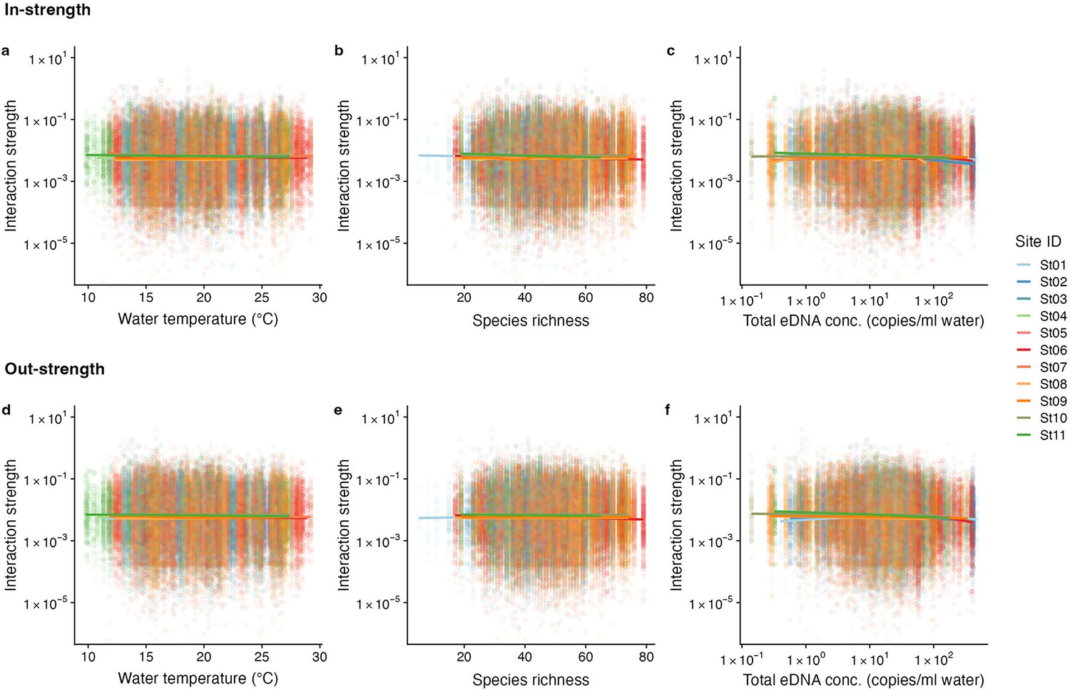
The relationship between interaction strengths and water temperature, species richness, and total DNA concentrations.
The panel shows the overall relationship between interaction strengths of the 50 dominant fish species and (a, d) water temperature, (b, e) species richness, and (c, f) total DNA concentration. The y-axis indicates the interaction strength between fish species quantified by the MDR S-map method. Note that the MDR S-map enables quantification of interaction strengths at each time point, and thus the number of data points is large (also true in Figure 3—figure supplement 3 and Figure 4—figure supplements 1 and 2). (a–c) Points indicate the species interactions that a focal species receives (i.e., in-strength), and (d–f) points indicate the species interactions that a focal species gives (i.e., out-strength). The line indicates the nonlinear regression line estimated by the general additive model. Colors of points and lines indicate the study site.
Figure 3—figure supplement 3
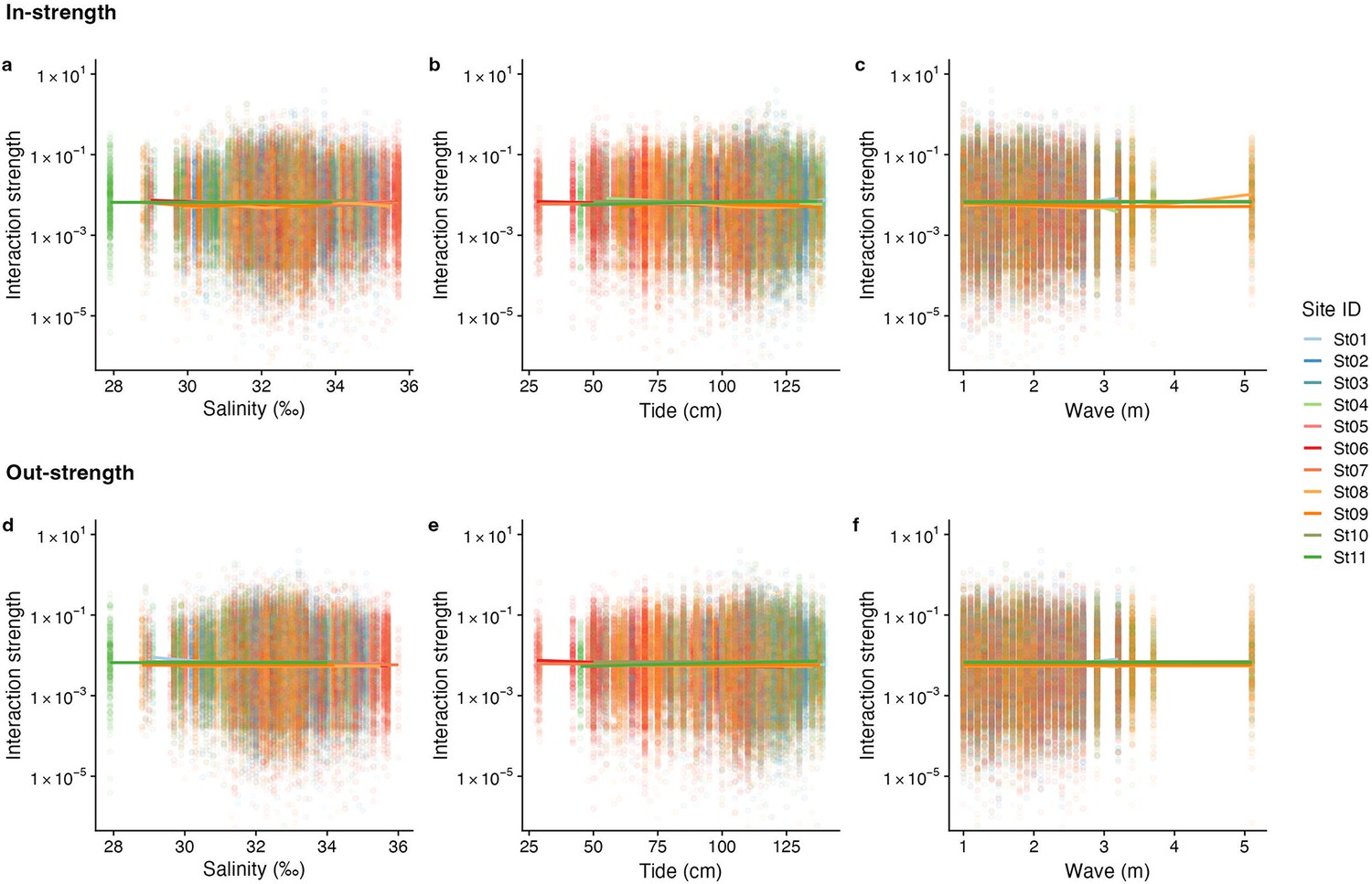
The relationship between interaction strengths and salinity, tide level, and wave.
The panel shows the overall relationship between interaction strengths of the 50 dominant fish species and (a, d) salinity, (b, e) tide level (cm), and (c, f) wave (m). The y-axis indicates the interaction strength between fish species quantified by the MDR S-map method. Note that the MDR S-map enables quantifications of interaction strengths at each time point, and thus the number of data points is large. (a–c) Points indicate the species interactions that a focal species receives (i.e., in-strength), and (d–f) points indicate the species interactions that a focal species gives (i.e., out-strength). The line indicates the nonlinear regression line estimated by the general additive model. Colors of points and lines indicate the study site.
Figure 4 with 2 supplements
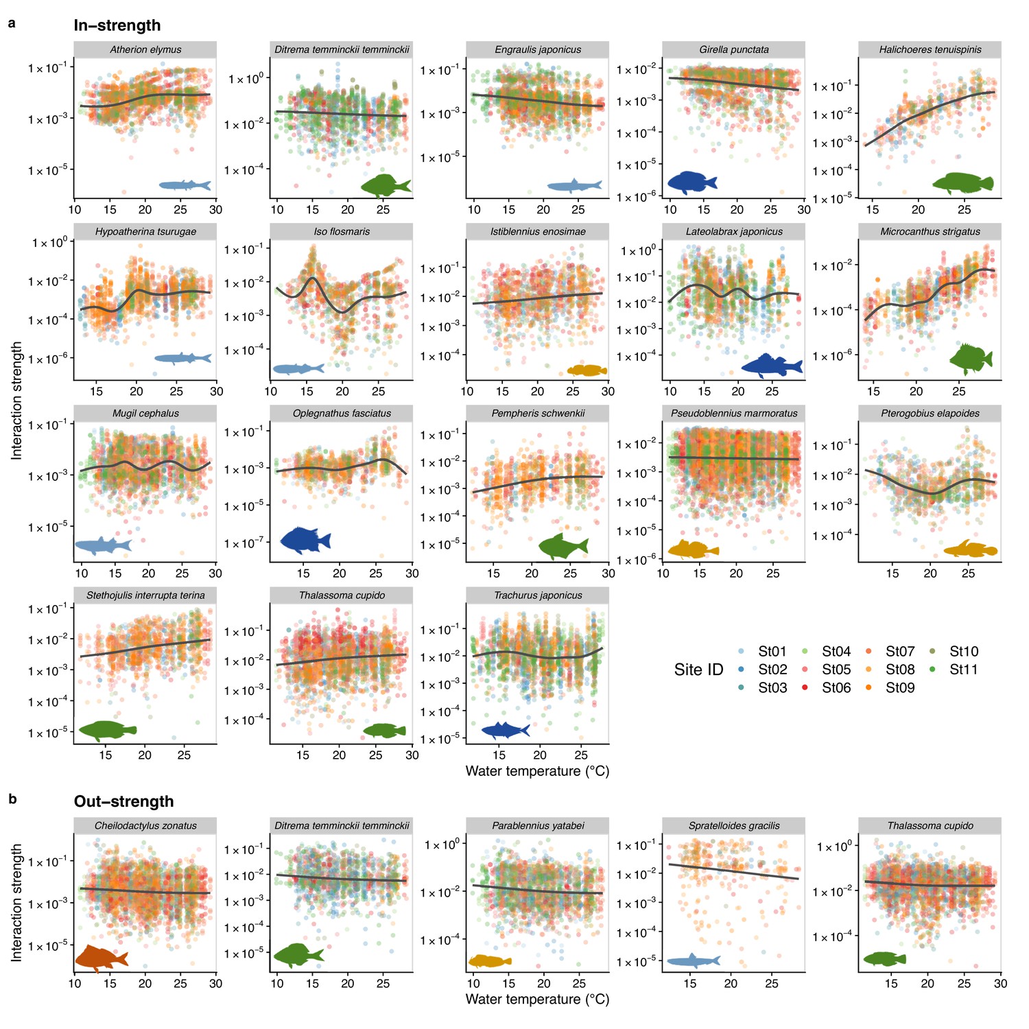
Temperature dependence of fish species interactions at the species level.
(a and b) show temperature effects on fish species interactions quantified by the MDR S-map method. Note that the MDR S-map enables quantifications of interaction strengths at each time point, and thus the number of data points is large. (a) Points indicate the species interactions that a focal species (indicated by the strip label and fish image) receives (i.e., in-strength). (b) Points indicate the species interactions that a focal species (indicated by the strip label and fish image) gives (i.e., out-strength). For (a) and (b), only fish species of which interactions are statistically clearly affected by water temperature are shown (to exclude fish species with relatively weak temperature effects, p < 0.0001 was used as a criterion here). Point color indicates the study site. Gray line is drawn by general additive model (GAM; the study sites were averaged for visualization purpose).
Figure 4—figure supplement 1
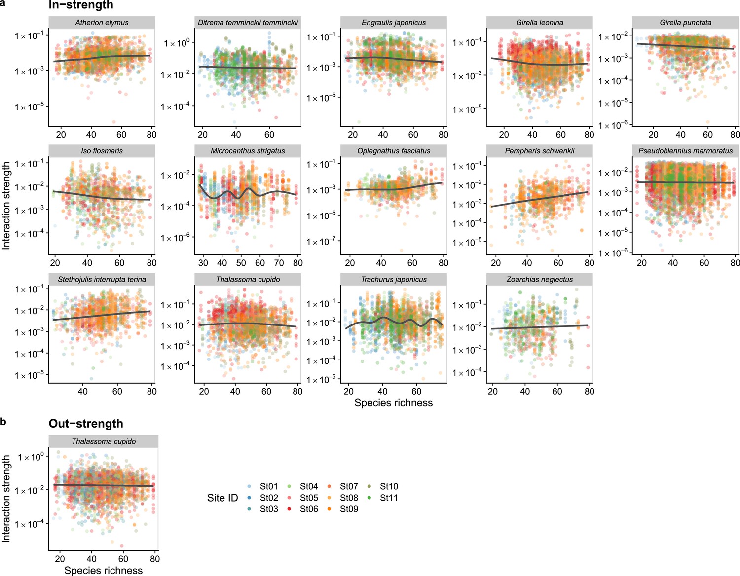
Dependence of fish species interactions on species richness at the fish species level.
(a and b) show effects of species richness on fish species interactions quantified by the MDR S-map method. (a) Points indicate the species interactions that a focal species (indicated by the strip label and fish image) receives (i.e., in-strength). (b) Points indicate the species interactions that a focal species (indicated by the strip label and fish image) gives (i.e., out-strength). For (a) and (b), only fish species of which interactions are statistically clearly affected by water temperature are shown (to exclude fish species with relatively weak temperature effects, p < 0.0001 was used as a criterion here). Point color indicates the study site. Gray line is drawn by general additive model (GAM; the study sites were averaged for visualization purpose).
Figure 4—figure supplement 2
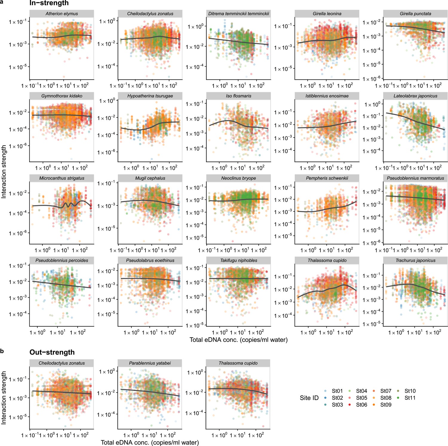
Dependence of fish species interactions on the total DNA concentration (an index of total fish abundance) at the species level.
(a and b) show effects of the total DNA concentrations on fish species interactions quantified by the MDR S-map method. (a) Points indicate the species interactions that a focal species (indicated by the strip label and fish image) receives (i.e., in-strength). (b) Points indicate the species interactions that a focal species (indicated by the strip label and fish image) gives (i.e., out-strength). For (a) and (b), only fish species of which interactions are statistically clearly affected by water temperature are shown (to exclude fish species with relatively weak temperature effects, p < 0.0001 was used as a criterion here). Point color indicates the study site. Gray line is drawn by general additive model (GAM; the study sites were averaged for visualization purpose).
Tables
Table 1
Primer sequences used in the present study.
| Primer information | Primer sequence (5′– 3′)*,†,‡, §,¶ | Length |
|---|---|---|
| 1st PCR primers | ||
| MiFish-U-forward | ACACTCTTTCCCTACACGACGCTCTTCCGATCT NNNNNN GTCGGTAAAACTCGTGCCAGC | 60 |
| MiFish-U-reverse | GTGACTGGAGTTCAGACGTGTGCTCTTCCGATCT NNNNNN CATAGTGGGGTATCTAATCCCAGTTTG | 67 |
| MiFish-E-forward-v2 | ACACTCTTTCCCTACACGACGCTCTTCCGATCT NNNNNN RGTTGGTAAATCTCGTGCCAGC | 61 |
| MiFish-E-reverse-v2 | GTGACTGGAGTTCAGACGTGTGCTCTTCCGATCT NNNNNN GCATAGTGGGGTATCTAATCCTAGTTTG | 68 |
| MiFish-U2-forward | ACACTCTTTCCCTACACGACGCTCTTCCGATCT NNNNNN GCCGGTAAAACTCGTGCC | 57 |
| MiFish-U2-reverse | GTGACTGGAGTTCAGACGTGTGCTCTTCCGATCT NNNNNN CATAGGAGGGTGTCTAATCCCCGTTTG | 67 |
| 2nd PCR primers | ||
| 2nd-PCR-forward | AATGATACGGCGACCACCGAGATCTACAC XXXXXXXX ACACTCTTTCCCTACACGACGCTCTTCCGATCT | 70 |
| 2nd-PCR-reverse | CAAGCAGAAGACGGCATACGAGAT XXXXXXXX GTGACTGGAGTTCAGACGTGTGCTCTTCCGATCT | 66 |
-
*
Normal characters indicate target-specific universal primers (i.e., MiFish primers).
-
†
The six random bases (Ns) in the middle of the 1st PCR primers were appended to enhance cluster separation on flow cells.
-
‡
Italic characters indicate Illumina sequencing primers.
-
§
X indicates index sequences to identify each sample.
-
¶
Underlined characters indicate P5/P7 adapter sequences for Illumina sequencing.
Additional files
-
Supplementary file 1
Supplementary information for eDNA metabarcoding and statistical analyses.
(a) List of species detected from MiFish environmental DNA (eDNA) metabarcoding with raw numbers of reads. (b) A faunal inventory of the coastal marine fishes of Chiba prefecture compiled from museum collections and literature surveys. Museum acronyms are Natural History Museum and Institute, Chiba (CBM) and its coastal branch (CHMH), National Museum of Nature and Science, Tokyo (NSMT), Kanagawa Prefectural Museum of Natural History (KPM), and Yokosuka City Museum (YCM). All references can be found in the footnote. (c) Top 20 fish–fish interactions based on UIC and their interpretations. (d) Results of GAMM between interaction strengths and environmental and ecological properties.
- https://cdn.elifesciences.org/articles/85795/elife-85795-supp1-v3.xlsx
-
Transparent reporting form
- https://cdn.elifesciences.org/articles/85795/elife-85795-transrepform1-v3.pdf
Download links
A two-part list of links to download the article, or parts of the article, in various formats.
Downloads (link to download the article as PDF)
Open citations (links to open the citations from this article in various online reference manager services)
Cite this article (links to download the citations from this article in formats compatible with various reference manager tools)
Temperature sensitivity of the interspecific interaction strength of coastal marine fish communities
eLife 12:RP85795.
https://doi.org/10.7554/eLife.85795.3


