Foxtrot migration and dynamic over-wintering range of an Arctic raptor
- Department of Migration, Max Planck Institute of Animal Behavior, Germany
- Leibniz Institute for Zoo and Wildlife Research, Germany
- Deutsches Zentrum für Luft- und Raumfahrt e.V. (DLR), Germany
- Institute of Plant and Animal Ecology, Russian Federation
- Institute of the Biological Problems of the North, Russian Federation
- Centre for the Advanced Study of Collective Behaviour, University of Konstanz, Germany
Figures
Figure 1 with 1 supplement
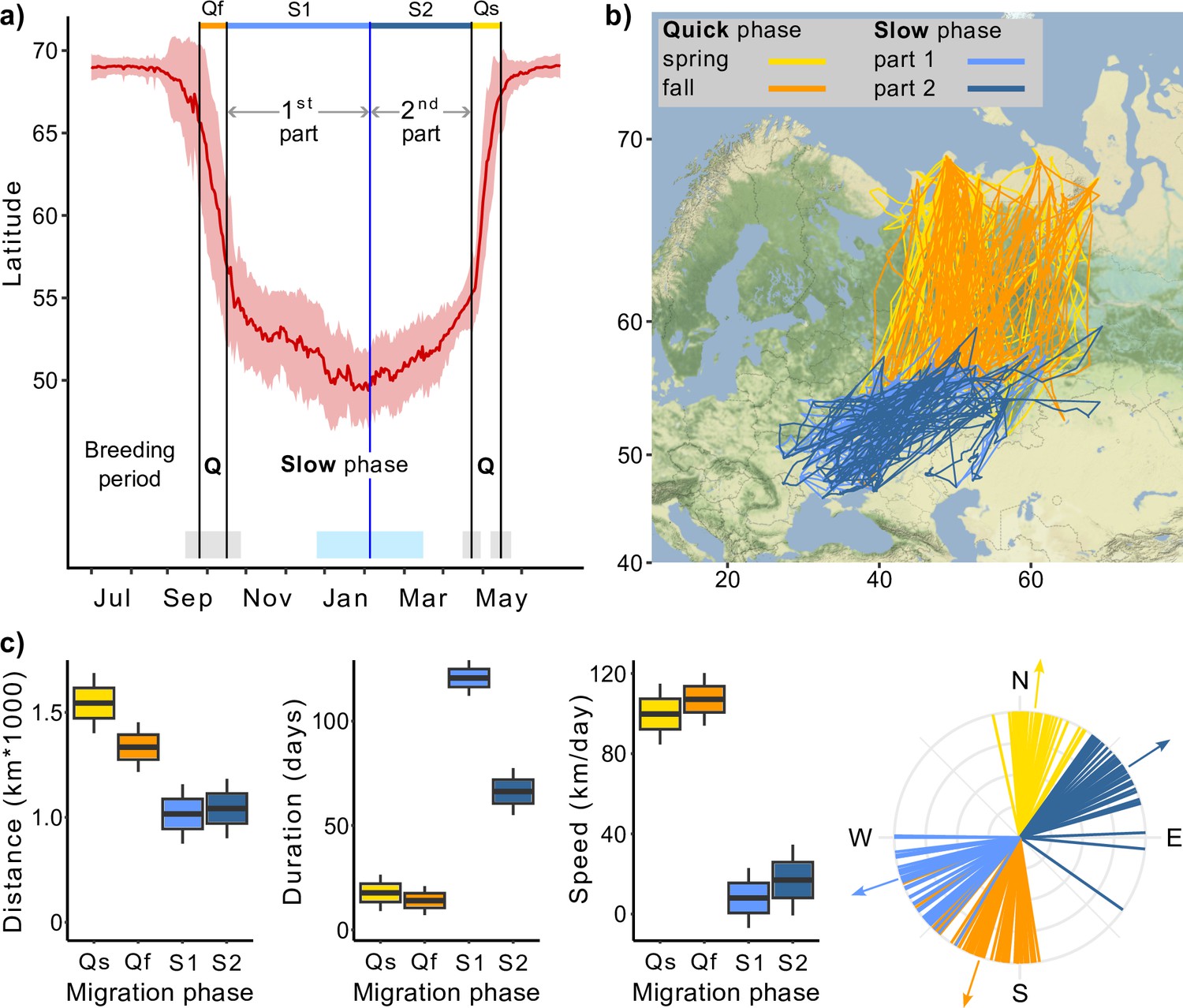
Migration of Rough-legged buzzards.
Q, quick phase; Qf, quick fall phase (orange); Qs, quick spring phase (yellow); S1, slow phase, first part (light blue); S2, slow phase, second part (dark blue). (a) Change in the latitude of 43 Rough-legged buzzards during the year, red line indicates mean latitude of all birds, black vertical lines indicate mean dates of start and end of the migration phases, blue vertical line indicates mean date of the minimum latitude. Gray, sky blue, and piggy pink shaded areas indicate standard deviation of the means. (b) Migration map. (c) Difference in the migration parameters between the migration phases. Lines on the direction plot (down, right) represent the mean value for each bird; arrows represent the mean direction for each phase. Boxes on the boxplots show the interquartile range, the whiskers are maximum and minimum values.
Figure 1—figure supplement 1
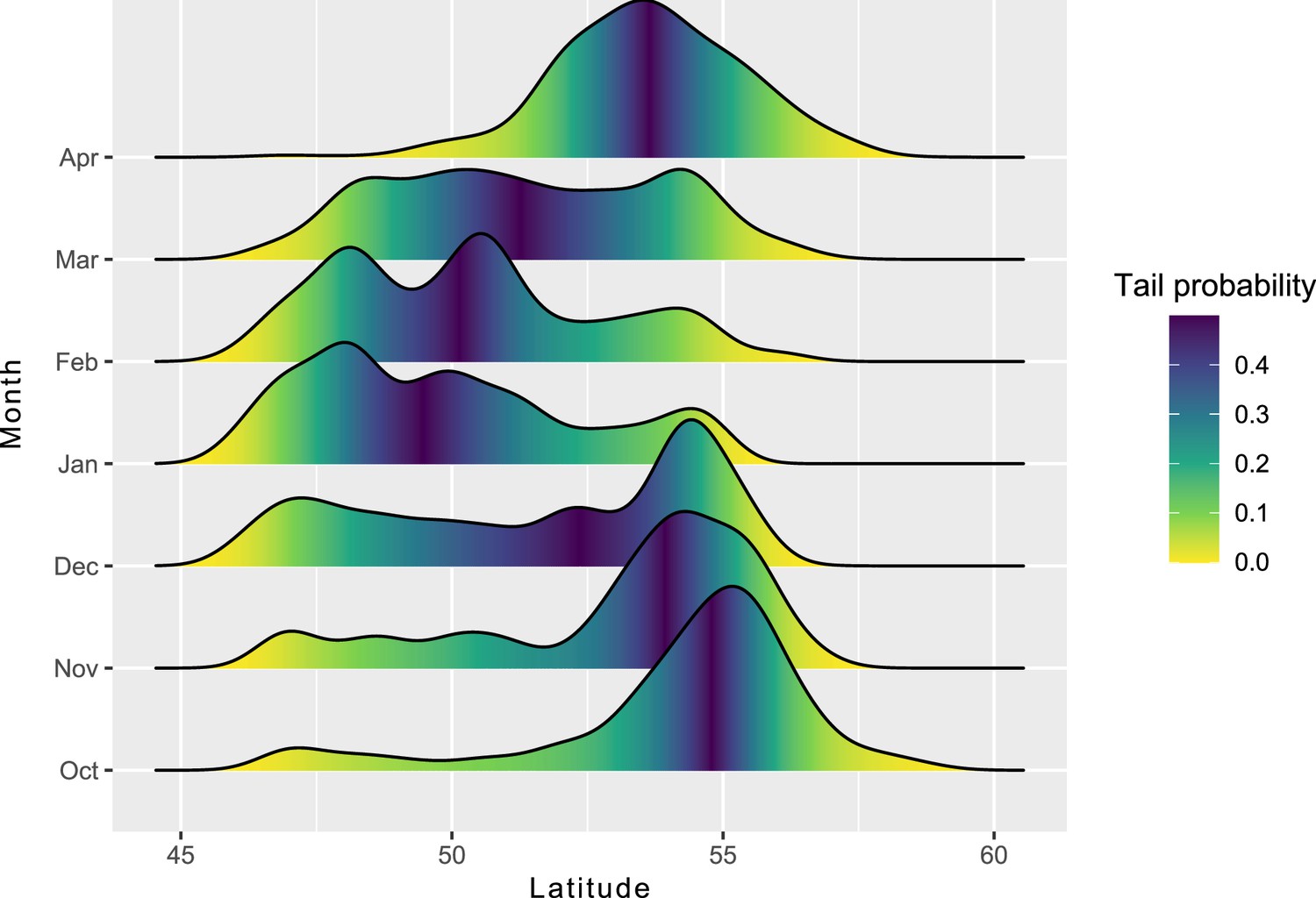
The distribution of latitudes of Rough-legged buzzards in different months.
Figure 2
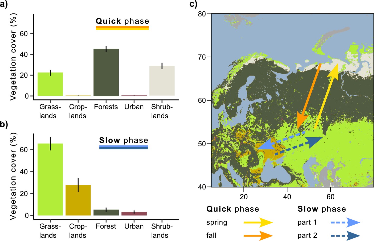
Vegetation land cover during quick and slow phases of the migration.
(a) Quick phase (spring and fall periods together). (b) Slow phase (first and second parts together). On both (a) and (b), the bars show the percentage of all mean daily positions annotated with the given vegetation type ± sd. (c) Migration map.
Figure 3 with 1 supplement
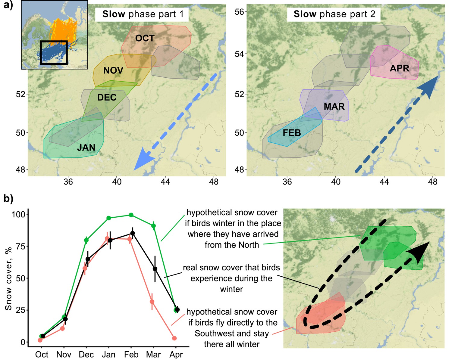
Snow cover conditions during the slow phase of the migration.
(a) 95% minimum convex polygons (MCPs) of Rough-legged buzzards during winter. Arrows indicate the direction of the movement across months. OCT, October; NOV, November; DEC, December; JAN, January; FEB, February; MAR, March; APR, April. (b) Snow cover conditions for the real situation (black) and two hypothetical situations – if birds spend the winter in the place where they arrived after the fall migration (green) and if birds fly directly to the southwest and stay there all winter (red). Dots represent mean values, error lines indicate standard deviations.
Figure 3—figure supplement 1
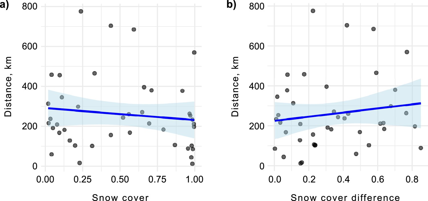
The distance between two consecutive monthly minimum convex polygons (MCPs) during the over-wintering period was not influenced by (a) snow cover extent on the first MCP (p=0.45) or (b) the difference in snow cover between two consecutive monthly MCPs (p=0.36).
Figure 4
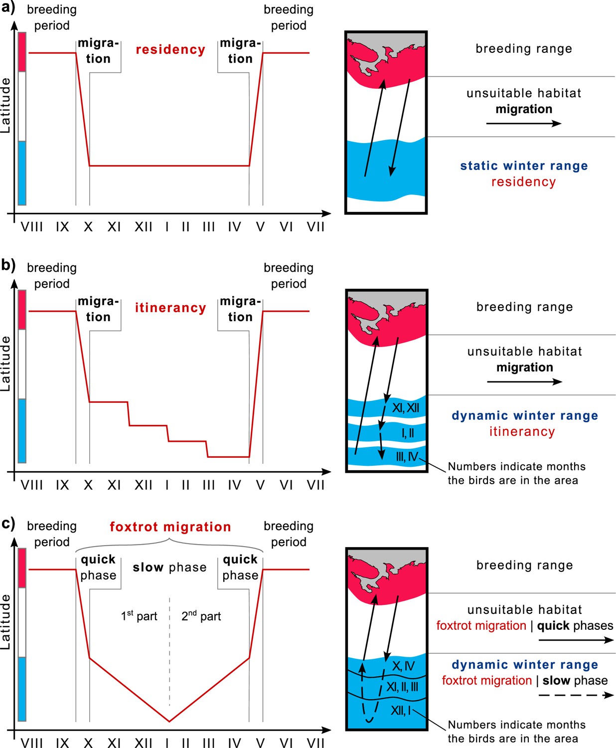
Winter strategies and over-wintering range scheme.
(a) Residency, (b) Itinerancy, and (c) Foxtrot migration. The color bar along the y-axis corresponds to the color coding of the habitats of the chart on the right.
Figure 5
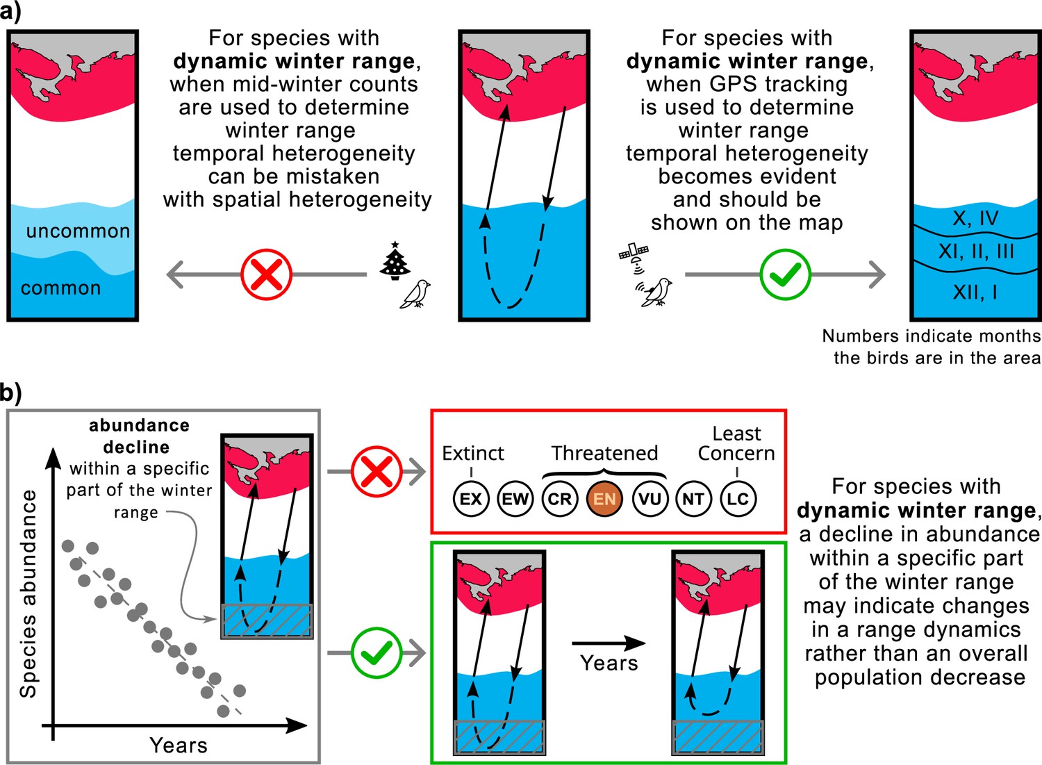
Mapping ranges and assessing population trends for the species with the dynamic over-wintering ranges.
(a) Mid-winter counts, often used to determine winter range, may give a misleading representation of the over-wintering range for species with dynamic range. (b) Changing the conservation status of a species based on reduced abundance in a particular area may not be appropriate for species with dynamic range. Red, breeding range; blue, winter range.
Tables
Table 1
Parameters of the Rough-legged buzzards’ migration (mean ± sd).
| Phase of migration | Sub-phase of migration | Distance (km) | Duration (days) | Speed (km/day) | Direction (°) |
|---|---|---|---|---|---|
| Quick | 1415 ± 50 | 15 ± 3 | 104 ± 6 | ||
| Spring | 1544 ± 72 | 18 ± 4 | 100 ± 8 | 7 ± 2 | |
| Fall | 1334 ± 59 | 14 ± 4 | 107 ± 7 | 198 ± 3 | |
| Slow | 1026 ± 55 | 100 ± 4 | 12 ± 7 | ||
| First phase | 1016 ± 71 | 121 ± 4 | 8 ± 7 | 251 ± 3 | |
| Second phase | 1042 ± 71 | 66 ± 6 | 17 ± 9 | 57 ± 2 |
Additional files
-
Supplementary file 1
Supplementary tables.
(a) Table S1. The relationship between latitude/longitude and the day of the year during quick and slow phases of migration. The likelihood ratio test compares two candidate models: with (‘~doy’) and without the day of the year (‘~1’) as a fixed factor. (b) Table S2. The relationship between latitude/longitude and the day of the year during quick and slow phases of migration. Linear mixed-effect model, fixed effects. The response variable – latitude/longitude. Fixed effect – the day of the year (‘doy’). Random effects – individuals and year. (c) Table S3. The relationship between latitude/longitude and the day of the year during quick and slow phases of migration. Linear mixed-effect model, random effects. The response variable – latitude/longitude. Fixed effect – the day of the year. Random effects – individuals (‘bird’) and year (‘year’). (d) Table S4. The difference between the distance of slow and quick migrations. Linear mixed-effect model, post hoc results. The response variable – distance (km). Fixed effect – the type of migrations. Results of the post hoc comparison. (e) Table S5. The difference between the duration of slow and quick migrations. Linear mixed-effect model, post hoc results. The response variable – duration (days). Fixed effect – the type of migrations. Results of the post hoc comparison. (f) Table S6. The difference between the speed of slow and quick migrations. Linear mixed-effect model, post hoc results. The response variable – speed (km/day). Fixed effect – the type of migrations. Results of the post hoc comparison. (g) Table S7. The difference between the direction of the spring and the second phase of the winter migration and between the autumn and the first phase of the winter migration (two models). Linear mixed-effect models, post hoc results. The response variable in both models – direction (deg). Fixed effect – the type of migrations. Results of the post hoc comparison. (h) Table S8. The relationship between migration distance and the sex of the birds. The likelihood ratio test compares two candidate models: with (‘~sex’) and without the sex (‘~1’) as a fixed factor. (i) Table S9. The difference between vegetation land cover types crossed during quick (fall and spring) and slow (winter) migrations. General linear mixed-effect models. Results are given on the logit scale. (j) Table S10. The difference between snow cover conditions in the real situation (‘Real’) and two and two hypothetical situations – if birds spend winter in the place where they have arrived after fall migration (‘Hyp stay’) and if birds fly directly to the Southwest and stay there all winter (‘Hyp SW’). General linear mixed-effect models. Results are given on the logit scale. Results of the post hoc comparison.
- https://cdn.elifesciences.org/articles/87668/elife-87668-supp1-v1.docx
-
MDAR checklist
- https://cdn.elifesciences.org/articles/87668/elife-87668-mdarchecklist1-v1.docx
Download links
A two-part list of links to download the article, or parts of the article, in various formats.
Downloads (link to download the article as PDF)
Open citations (links to open the citations from this article in various online reference manager services)
Cite this article (links to download the citations from this article in formats compatible with various reference manager tools)
Foxtrot migration and dynamic over-wintering range of an Arctic raptor
eLife 12:RP87668.
https://doi.org/10.7554/eLife.87668.4


