Meta-analysis reveals glucocorticoid levels reflect variation in metabolic rate, not ‘stress’
- Instituto de Investigación en Recursos Cinegéticos (IREC), CSIC-UCLM-JCC, Spain
- Instituto Pirenaico de Ecologia (IPE), CSIC, Avda. Nuestra Señora de la Victoria, Spain
- University of Groningen, Netherlands
Figures
Box 1—figure 1
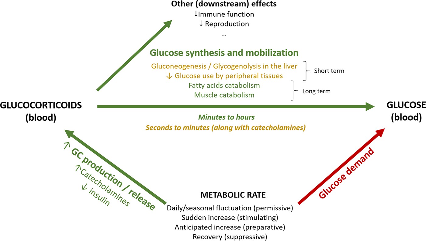
Schematic representation of the association between metabolic rate and plasma levels of glucocorticoids and glucose.
Green arrows represent increasing effects, whereas red arrows represent reducing effects.
Figure 1 with 1 supplement
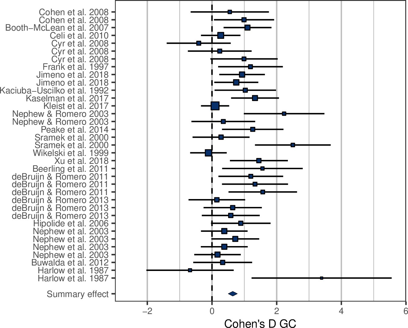
Forest plot showing the glucocorticoid (GC) effect sizes (Cohen’s D ± 95% CI) associated with experimental manipulations of metabolic rate, grouped by treatment group and study.
Area of squares is proportional to the experiment sample size (1/s.e.).
Figure 1—figure supplement 1

Forest plot showing the metabolic rate (MR) effect sizes (Cohen’s D ± 95% CI) associated with experimental manipulations of MR, grouped by treatment group and study.
Area of squares is proportional to the experiment sample size (1/s.e.).
Figure 2 with 2 supplements
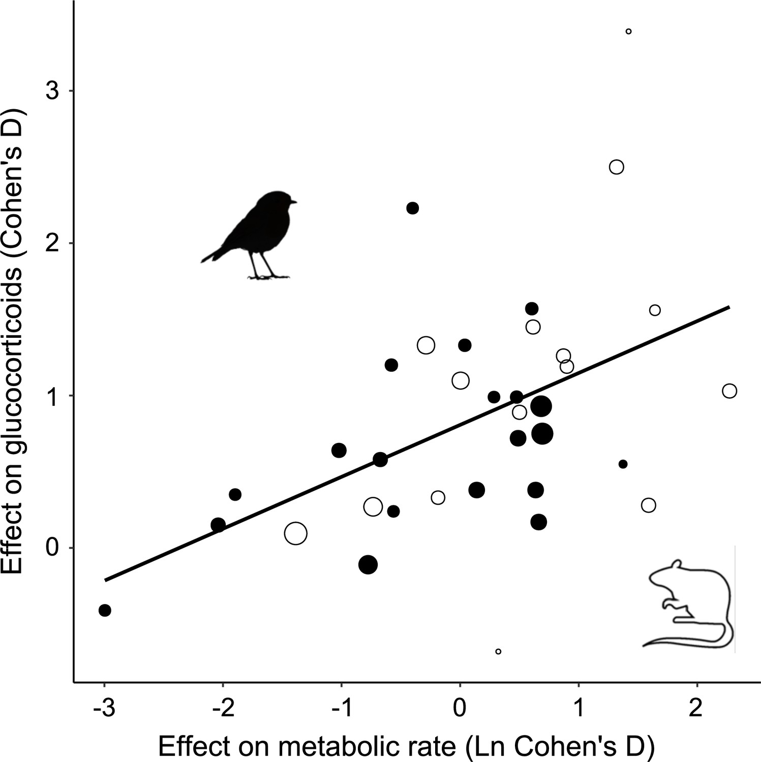
Glucocorticoid (GC) effect size (Cohen´s D) increases with increasing metabolic rate effect size similarly in studies of mammals (open circles) and birds (closed circles).
Area of dots is proportional to the experiment sample size (i.e. square root of the number of individuals in which GCs were measured).
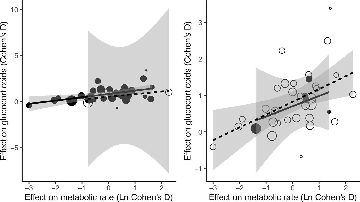
Figure 2—figure supplement 1
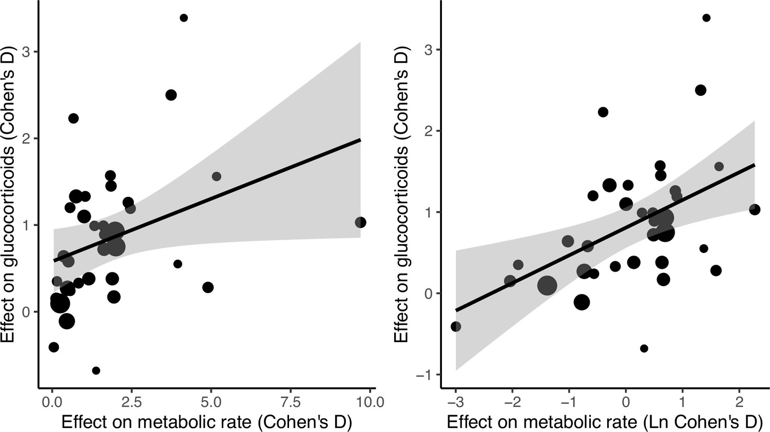
Relationship between metabolic rate and glucocorticoid effect sizes (Cohen’s D) across studies.
Panels show the association without ln-transforming metabolic rate effect sizes (left panel) and when ln-transforming them (right panel). Size of dots is proportional to the experiment sample size (i.e. square root of the number of individuals in which glucocorticoids were measured). Shaded areas represent 95% CI. Note that the number of data points in the graph is higher than the number of studies as some of the studies included multiple experimental treatments (Study ID was included as random factor in statistical analyses).
Figure 2—figure supplement 2
Relationship between metabolic rate and glucocorticoid effect sizes (Cohen’s D) across studies as a function of before/after effect (left panel; open circles and dashed line for studies including a time effect; closed circles and continuous line for studies not including a time effect; see ‘Materials and methods’) and experiment/control effect (right panel; open circles and dashed line for studies including within-individual variation; closed circles and continuous line for studies not including within-individual variation).
Size of dots is proportional to the experiment sample size (i.e. square root of the number of individuals in which glucocorticoids were measured). Shaded areas represent 95% CI. Note that the number of data points in the graph is higher than the number of studies as some of the studies included multiple experimental treatments (Study ID was included as random factor in statistical analyses). Before/after effect and experiment/control effect results should be interpreted with caution as most studies do include within-individual variation and do not include time effect.
Tables
Table 1
Meta regression model testing the association between metabolic rate (MR) effect sizes and glucocorticoid effect sizes.
| Estimate | s.e. | Z | p | 95% CI | |
|---|---|---|---|---|---|
| Intercept | 0.72 | 0.11 | 6.40 | <0.0001 | 0.50–0.95 |
| MR effect size (ln) | 0.31 | 0.10 | 2.94 | 0.003 | 0.10–0.51 |
-
Variance components: Study.ID (Sigma^2)– Estimate = 0.00, sqrt = 0.00, n = 21.
-
Residual heterogeneity: QE(df = 33) = 28.40, p=0.70.
-
Test of moderators: QM(df = 1) = 8.64, p=0.003.
Table 2
Table showing the main effects of all variables considered (metabolic rate [MR], taxa, time effect, within-individual variation, metabolic variable, and treatment type) to modulate glucocorticoid effect sizes across studies.
Full models are shown in Supplementary file 4.
| Variable | p |
|---|---|
| MR effect size (ln) | 0.003 |
| Taxa | 0.63 |
| Before/after | 0.49 |
| Experiment/control | 0.68 |
| Metabolic variable | 0.94 |
| Treatment type | |
| Treat. 2 | 0.93 |
| Treat. 3 | 0.60 |
Author response table 1
Meta regression model testing the association between metabolic rate (MR) effect sizes and glucocorticoid effect sizes.
| Estimate | s.e. | z | P | 95% C.I.. | |
|---|---|---|---|---|---|
| Intercept | 0.76 | 0.11 | 7.20 | < 0.0001 | 0.55-0.96 |
| MR effect size (In) | 0.32 | 0.10 | 2.97 | 0.003 | 0.11-0.52 |
| Variance components: outer factor: Lab(N=16), inner factor: Study.ID (N=21). tau^2- Estimate = 0.02, sqrt = 0.1 | |||||
| Residual heterogeneity: QE(df=33)=28.26,p=0.70 | |||||
| Test of moderators: QM(df=1)=8.83,p=0.003 |
Author response table 2
Meta regression model (quantitative approach) testing the effect of (a) Taxa, (b) Before / after effect, (c) Experiment / control effect, (d) Use of Metabolic Rate or Heart Rate as metabolic variable and (e) Treatment type, on the association between metabolic rate (MR) and glucocorticoid effect sizes across studies.
| (a) | Estimate | s.e. | z | P | 95% C.I. |
|---|---|---|---|---|---|
| Intercept | 0.72 | 0.11 | 6.30 | < 0.0001 | 0.50-0.95 |
| MR effect size (In) | 0.30 | 0.11 | 2.75 | 0.006 | 0.09-0.52 |
| Taxa (mammal) | 0.07 | 0.23 | 0.33 | 0.74 | -0.38-0.54 |
| MR : Taxa | 0.16 | 0.22 | 0.71 | 0.48 | -0.28-0.59 |
| Variance components: outer factor: Lab (N=16), inner factor: Study. ID (N=21). tau^2- Estimate = 0.00, sqrt = 0.09 | |||||
| Residual heterogeneity: QE(df=31)=27.47,p=0.65 | |||||
| Test of moderators: QM(df=3)=9.53,p=0.023 | |||||
| (b) | Estimate | s.e. | z | P | 95% C.I. |
| Intercept | 0.77 | 0.10 | 7.69 | < 0.0001 | 0.57-0.96 |
| MR effect size (ln) | 0.32 | 0.11 | 3.00 | 0.002 | 0.11-0.54 |
| Before / after effect (yes) | -0.30 | 0.38 | -0.79 | 0.43 | -1.06-0.45 |
| MR : Time effect | -0.00 | 0.31 | 0.05 | 0.96 | -0.59-0.62 |
| Variance components: Lab (N=16), inner factor: Study.ID (N=21). tau^2 - Estimate = 0.03, sqrt = 0.16 | |||||
| Residual heterogeneity: QE(df=31)=27.72,p=0.64 | |||||
| Test of moderators: QM(df=3)=9.39,p=0.024 | |||||
| (c) | Estimate | s.e. | z | P | 95% C.I. |
| Intercept | 0.76 | 0.10 | 7.51 | < 0.0001 | 0.56-0.96 |
| MR effect size (ln) | 0.32 | 0.11 | 2.97 | 0.003 | 0.11-0.52 |
| Exp./ control effect (yes) | 0.08 | 0.31 | 0.25 | 0.80 | -0.53-0.69 |
| MR : Exp. / control effect | -0.05 | 0.32 | -0.00 | 0.99 | -0.62-0.62 |
| Variance components: Lab (N=16), inner factor: Study.ID (N=21). tau^2- Estimate = 0.02, sqrt = 0.15 | |||||
| Residual heterogeneity: QE(df=31)=28.18,p=0.61 | |||||
| Test of moderators: QM(df=3)=8.88,p=0.030 | |||||
| (d) | Estimate | s.e. | P | 95% C.I. | |
| Intercept | 0.76 | 0.11 | 7.12 | < 0.0001 | 0.55-0.97 |
| MR effect size (ln) | 0.34 | 0.11 | 3.00 | 0.003 | 0.12-0.56 |
| Met. variable (HR) | 0.15 | 0.22 | 0.68 | 0.49 | -0.28-0.59 |
| MR : Met. variable | 0.01 | 0.23 | 0.06 | 0.96 | -0.43-0.46 |
| Variance components: outer factor: Lab (N=16), inner factor: Study.ID (N=21). tau^2- Estimate = 0.03, sqrt = 0.16 | |||||
| Residual heterogeneity: QE(df=31)=28.03,p=0.62 | |||||
| Test of moderators: QM(df=3)=9.21,p=0.027 | |||||
| e) | Estimate | s.e. | z | P | 95% C.I. |
| Intercept | 0.82 | 0.20 | 4.09 | < 0.0001 | 0.43-1.21 |
| MR effect size (In) | 0.26 | 0.20 | 1.30 | 0.19 | -0.13-0.64 |
| Treat. Type 2 | 0.01 | 0.29 | 0.02 | 0.98 | -0.57-0.58 |
| Treat. Type 3 | -0.20 | 0.32 | -0.62 | 0.53 | -0.81-0.42 |
| MR: Treat. Type 2 | 0.09 | 0.27 | 0.34 | 0.74 | -0.44-0.62 |
| MR: Treat. Type 3 | 0.08 | 0.29 | 0.28 | 0.78 | -0.49-0.66 |
| Variance components: Lab (N=16), inner factor: Study.ID (N=21). tau^2- Estimate = 0.04, sqrt = 0.20 | |||||
| Residual heterogeneity: QE(df=29)=27.77,p=0.53 | |||||
| Test of moderators: QM(df=5)=9.32,p=0.097 |
Additional files
-
Supplementary file 1
Study selection steps and number of studies found.
- https://cdn.elifesciences.org/articles/88205/elife-88205-supp1-v1.docx
-
Supplementary file 2
Table showing the information extracted from each study included in the meta-analysis.
Studies included in the meta analysis: Cohen et al., 2008; Booth-McLean et al., 2007; Celi et al., 2010; Cyr et al., 2008; Frank et al., 1997; Jimeno et al., 2018; Kaciuba-Uscilko et al., 1992; Keselman et al., 2017; Kleist et al., 2017; Nephew and Romero, 2003; Peake et al., 2014; Srámek et al., 2000; Wikelski et al., 1999; Xu et al., 2018; Beerling et al., 2011; de Bruijn and Romero, 2011; de Bruijn and Romero, 2013; Hipólide et al., 2006; Nephew et al., 2003; Buwalda et al., 2012; Harlow et al., 1987.
- https://cdn.elifesciences.org/articles/88205/elife-88205-supp2-v1.csv
-
Supplementary file 3
Effect size calculations.
The document Includes one sheet per study with the data extracted, the part of the article it was extracted from, and the effect size calculations and results further included in the meta analysis and Supplementary file 2.
- https://cdn.elifesciences.org/articles/88205/elife-88205-supp3-v1.xlsx
-
Supplementary file 4
Meta-regression model (quantitative approach) testing the effect of (a) taxa, (b) before/after effect, (c) experiment/control effect, (d) use of metabolic rate (MR) or heart rate as metabolic variable, and (e) treatment type, on the association between MR and glucocorticoid effect sizes across studies.
- https://cdn.elifesciences.org/articles/88205/elife-88205-supp4-v1.docx
-
MDAR checklist
- https://cdn.elifesciences.org/articles/88205/elife-88205-mdarchecklist1-v1.docx
Download links
A two-part list of links to download the article, or parts of the article, in various formats.
Downloads (link to download the article as PDF)
Open citations (links to open the citations from this article in various online reference manager services)
Cite this article (links to download the citations from this article in formats compatible with various reference manager tools)
Meta-analysis reveals glucocorticoid levels reflect variation in metabolic rate, not ‘stress’
eLife 12:RP88205.
https://doi.org/10.7554/eLife.88205.3


