Figures and data
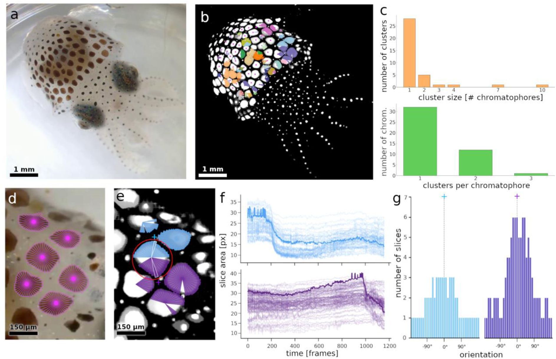
Identification and characterization of putative chromatophore motor units in E. berryi.
a) Example HD-video frame extracted from a E. berryi recording. b) Visual representation of presumed motor units. Colors represent motion clusters of chromatophore slices grouped together by covariation using the HDBSCAN algorithm. Clusters represent presumed motor units. c) Number of chromatophores per cluster size, and frequency of chromatophores belonging to multiple clusters. d) Zoom on the frame shown in a, with detected slices overlaid in magenta. e) Zoom on two overlapping motor units from b. The central chromatophore (red circle) contributes slices to both the blue and the purple clusters. Cluster centers of mass, calculated from the epicenters of the chromatophores belonging to each cluster, are shown as colored crosses. f) Surface areas of slices belonging to each cluster over time. In bold, the surface areas of the slices highlighted in white in e. g) Distribution of slice orientations relative to the motor unit’s center of mass.
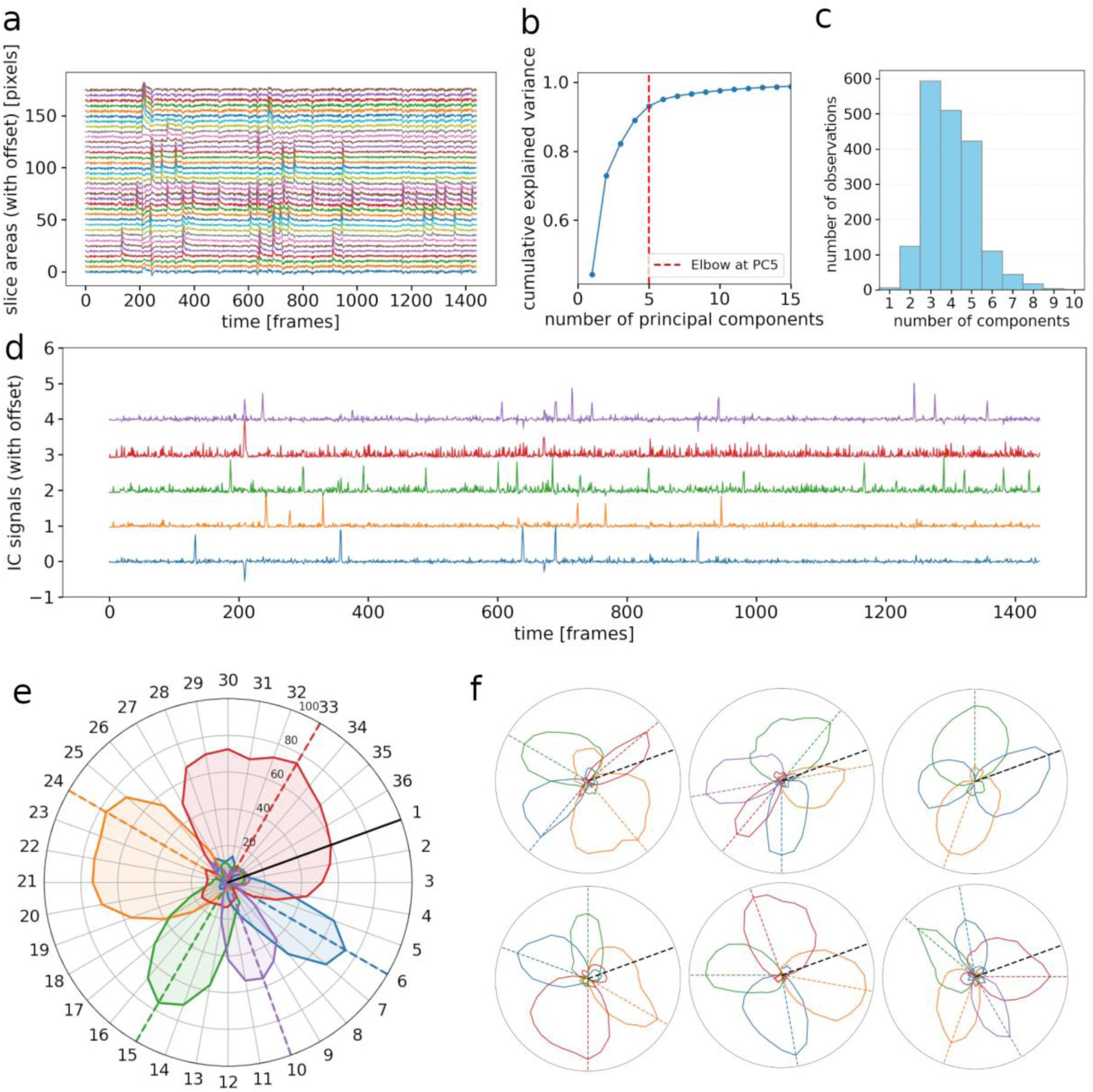
Multiple innervation of individual chromatophores.
a) Activity traces (surface area as functions of time) of 36 polar slices from a single chromatophore, offset vertically pairwise by 5 pixels for clarity. Each trace represents the positive, detrended change in surface area over time, highlighting expansion dynamics while excluding negative (contraction) phases. b) Cumulative explained variance plot for Principal Component Analysis. Relationship between number of principal components and explained variance, with PCs ranked by decreasing contribution. Red stippled line at PC corresponding to greatest slope change (see Methods) (here PC5). c) Histogram showing the number of principal components identified per chromatophore across the dataset. d) Independent sources acting on the 36 slices of a single chromatophore, extracted with Independent Component Analysis. In this case, the chromatophore is controlled by 5 independent sources that likely correspond to 5 distinct motor neurons. e) Polar plot representing the influence of each source (motor neuron activity) on each slice. Black line indicates the first radial slice; influence of a source on a slice expressed in % (radial scale). f) Examples of PCA-ICA analyses run on six other chromatophores.
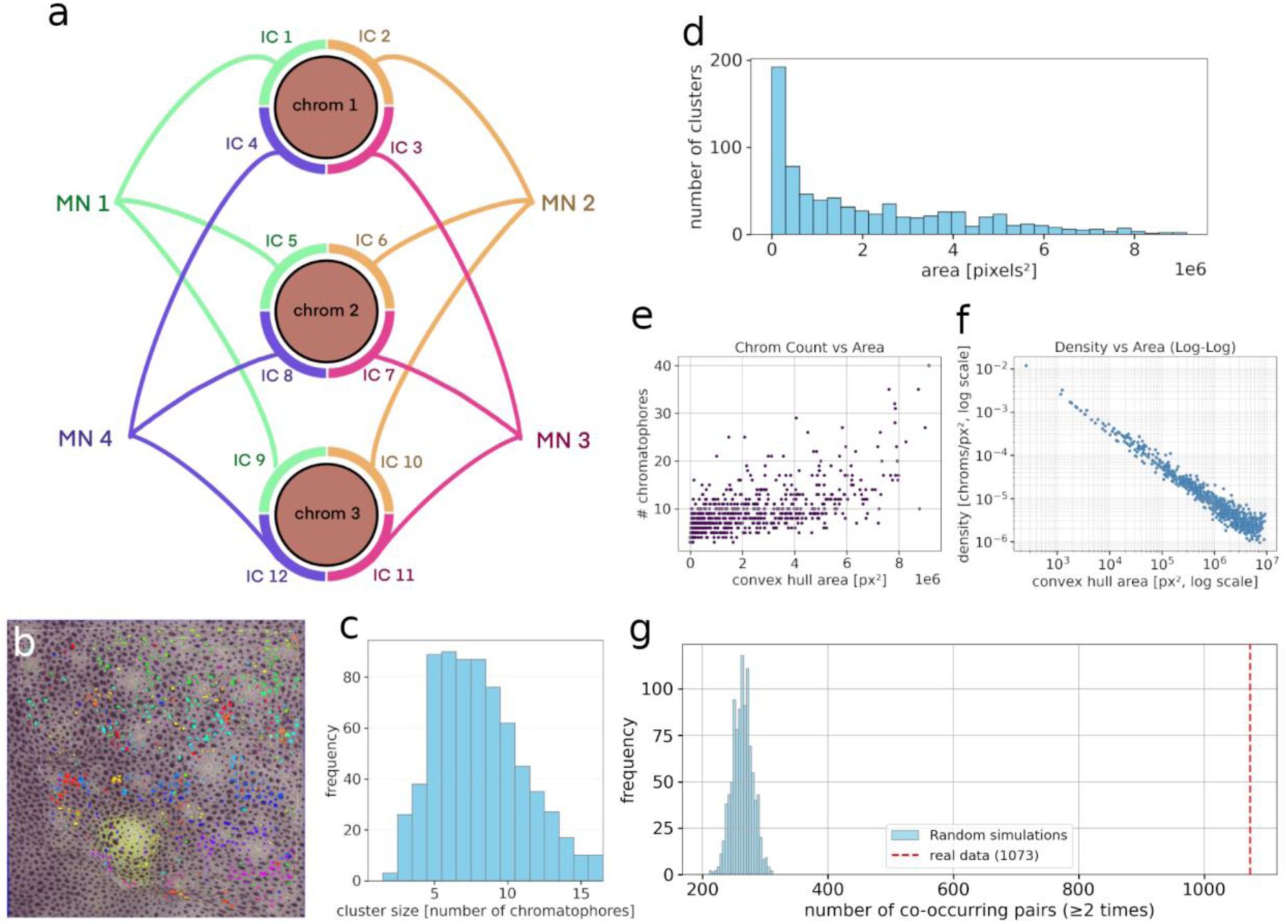
Identification of putative motor units.
a) Schematic representation of derived chromatophore innervation by motor neurons. Each chromatophore is depicted as a circle, with arcs around them representing independent components identified by ICA, each interpreted as corresponding to the zone of influence of a single motor neuron on that particular chromatophore. One goal of this clustering was to reveal shared chromatophore innervation and thus, motor units. Colors and lines connecting IC arcs indicate that they belong to the same motor unit, highlighting the shared innervation pattern across multiple chromatophores. b) A small number of clusters of size 3 to 5 are mapped back on the original image for visualisation. c) Distribution of cluster size (size in number of IC). d) Distribution of cluster convex hull areas, showing a right-skewed profile with most clusters occupying smaller areas. All values are reported in pixel² (px²); note that the main text reports corresponding measurements in µm² after conversion (10 pixels = 1 µm, thus 1 px² = 0.01 µm²). e) Relationship between chromatophore count and convex hull area for each cluster. f) Chromatophore density (chromatophores per pixel²) as a function of convex hull area, plotted on a log-log scale. The inverse relationship reflects decreasing density in larger clusters. g) Histogram showing the distribution of second-order co-occurrence counts—defined as the number of chromatophore pairs co-occurring in at least two clusters—across 1000 randomised datasets (blue). Randomisations preserved both the number of clusters and the number of memberships per chromatophore. The red dashed line indicates the observed experimental value, significantly higher than expected by chance.
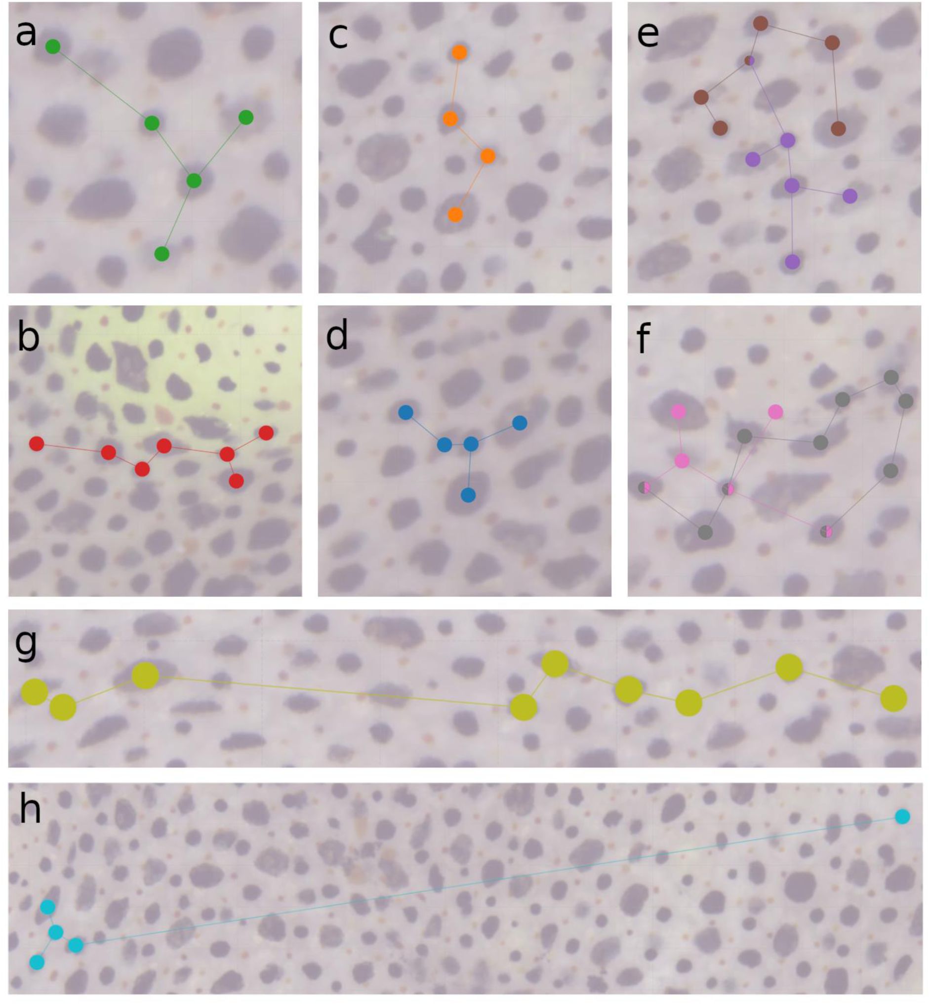
Spatial organization of putative motor units.
Chromatophores belonging to the same correlated-motion cluster, or putative MU, are shown as colored dots connected by lines. a-d) Compact clusters. e-f) Overlapping clusters with shared chromatophores. g) Elongated cluster with a linear structure. h) Mixed profile featuring a core group of adjacent chromatophores connected to a single, distant chromatophore.
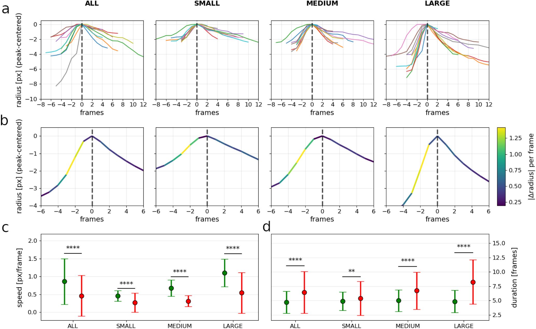
Composite summary of chromatophore slices expansion–contraction dynamics.
Events are first filtered to remove very small peaks (expansion amplitude ≤ 15% of the observed amplitude range). Remaining events are split by expansion amplitude percentiles: SMALL = lower tail, MEDIUM = central band, LARGE = upper tail. Within each tail band, outliers in either amplitude or speed are removed using Tukey’s IQR rule, and statistics are computed on the remaining events (see Methods). a) Peak-aligned event segments (10 randomly selected events per column) for each group. Traces are shifted to align at the peak (t=0). Same y calibration in the four panels. b) Mean event profile for each size group, where each segment is color-coded by instantaneous size change (|Δradius| for pairs of consecutive frames); LUT at right. Same y calibration in the four panels c) Means ± SDs of chromatophore size change (px/frame) for expansion (green) and contraction (red) phases. Statistical significance evaluated using paired t-tests between expansion and contraction phases (n = 2157 event pairs). Asterisks indicate significant paired differences p < 0.05 (*), p < 0.01 (**), p < 0.001 (***), and p < 0.0001 (****). d) Same as in c but for event duration (in frames).
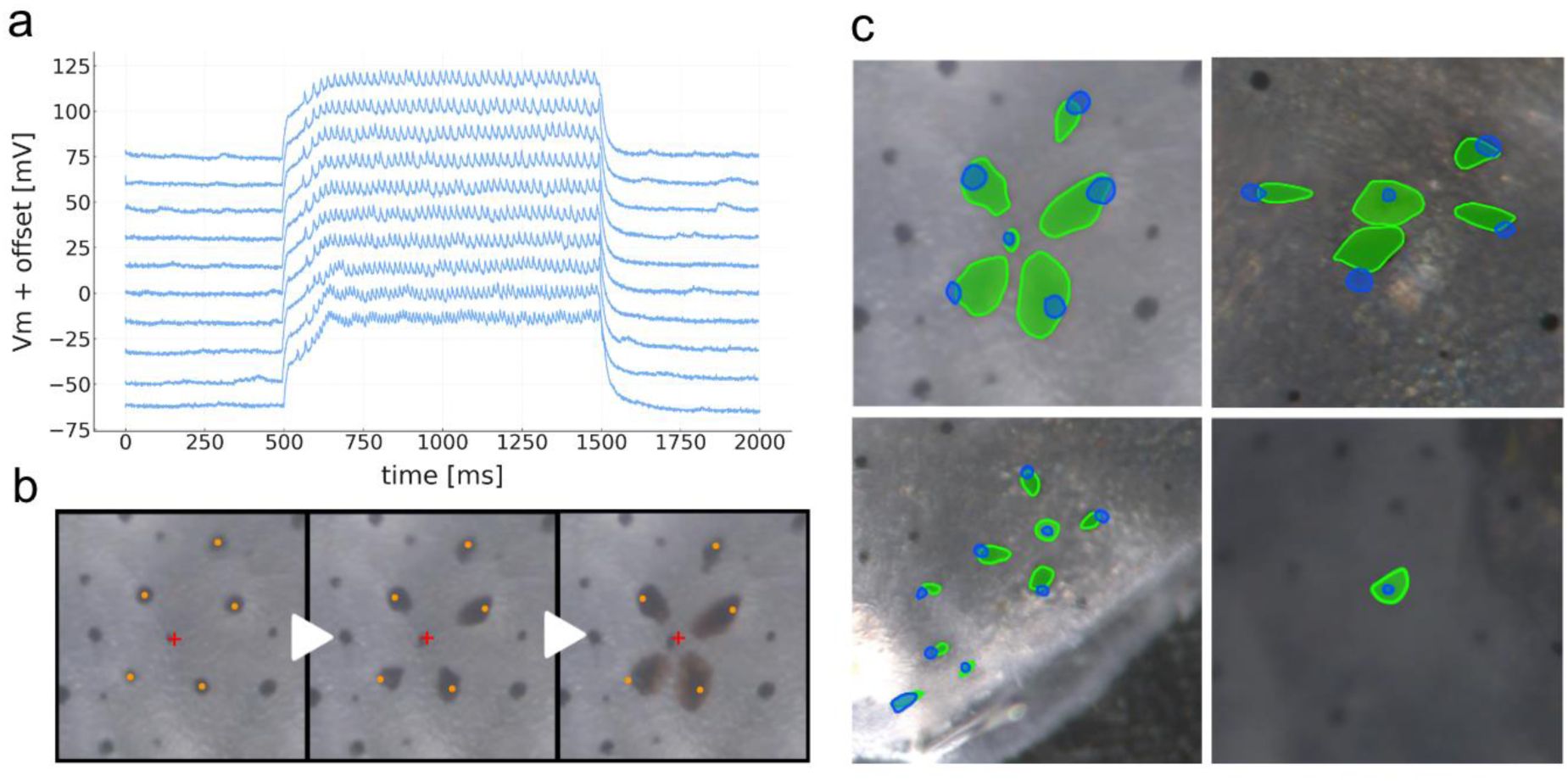
Patch clamp stimulation of chromatophore-lobe motor neuron.
a) “Patch-clamp recordings from a chromatophore-lobe motor neuron. Ten consecutive sweeps are shown, vertically offset for clarity and downsampled x4 (from 100 to 25 kHz). b) Sequence of video stills showing chromatophore expansion elicited by stimulation of the same motor neuron as in a. In orange, chromatophore epicenters, defined as the center of mass at the frame where the chromatophore is in its most contracted state. Each chromatophore expands anisotropically toward a common center of innervation (approximated as a red cross). c) Composite images showing chromatophore outlines before (blue) and during stimulation (green). The first three examples display anisotropic expansion across several chromatophores within a single motor unit—the first example is the same motor unit shown in a–b. The last example shows isotropic expansion of a motor unit composed of a single chromatophore.
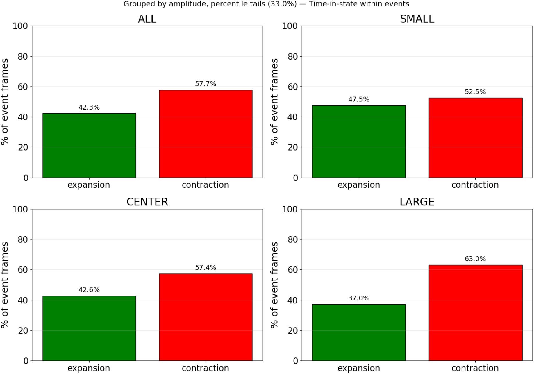
Relative temporal composition of chromatophore events across amplitude groups.
For each amplitude category (SMALL, MEDIUM, LARGE), the proportion of frames spent in the expansion (green) versus contraction (red) phase was computed across all valid events (n = 2157). Percentages were calculated relative to the total duration of each event (expansion + contraction). This analysis corresponds to the same dataset shown in Fig. 5.
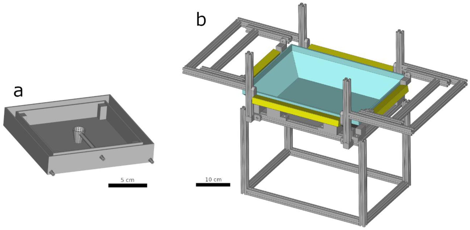
Designs of experimental arenas.
a) Arena for Euprymna berryi hatchlings. b) Rig for Sepia officinalis. Four adjustable LED lamps in yellow. Transparent tank in cyan. Structure in gray.
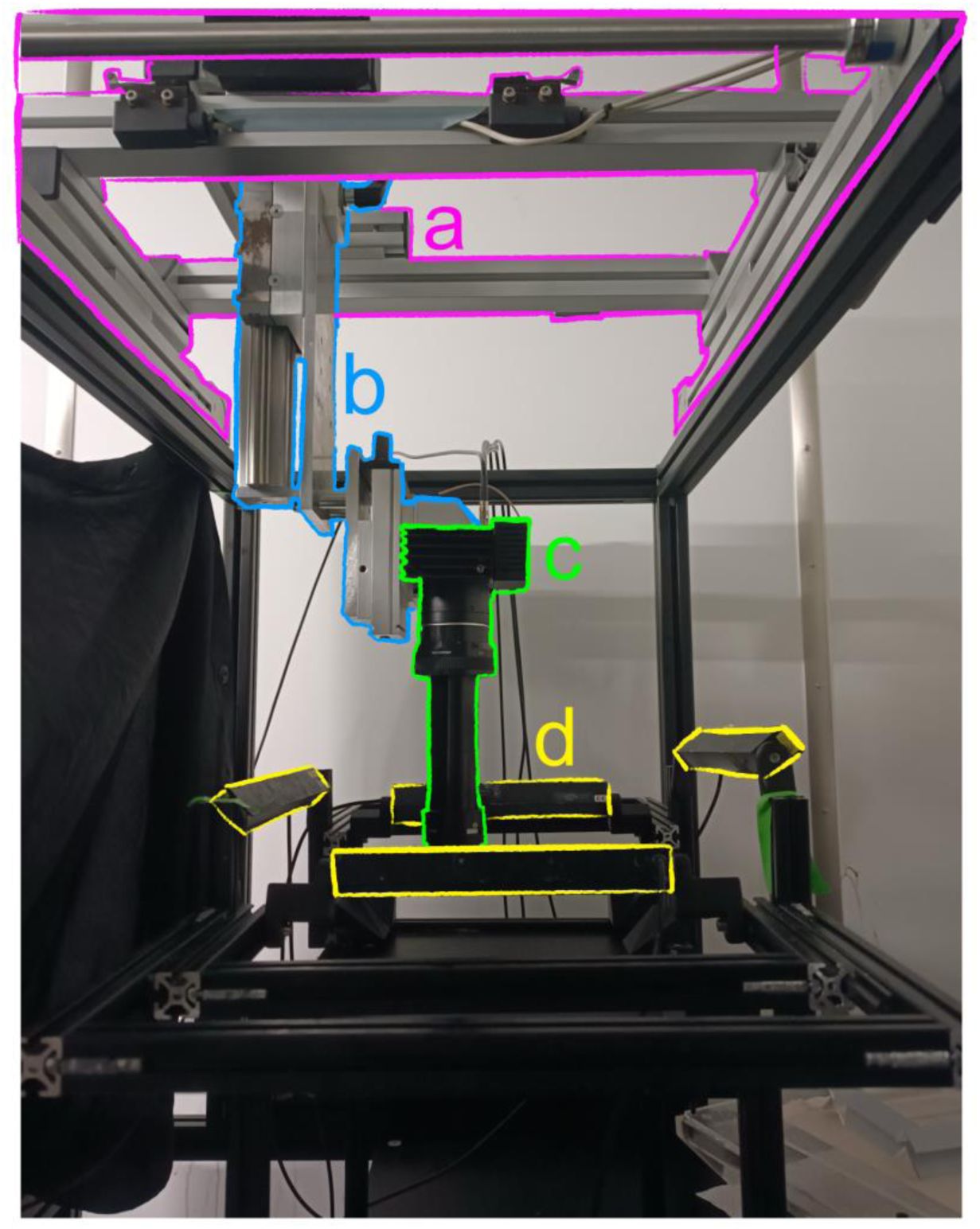
Sepia filming setup.
a) Remotely controlled linear rails. b) Z-axis manual translation stage. c) Camera and lens. d) LED lights.
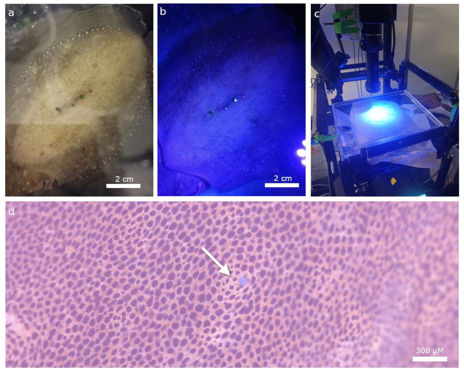
Visible implant elastomer tagging.
a) Sepia officinalis marked at the center of the mantle with tags of various colors in a row. b) Marked animal under fluorescent light. c) Fluorescent lamp mounted next to the camera on the filming rig. d) Footage captured by the high-resolution camera. Close-up on the blue fluorescent tag indicated by an arrow.
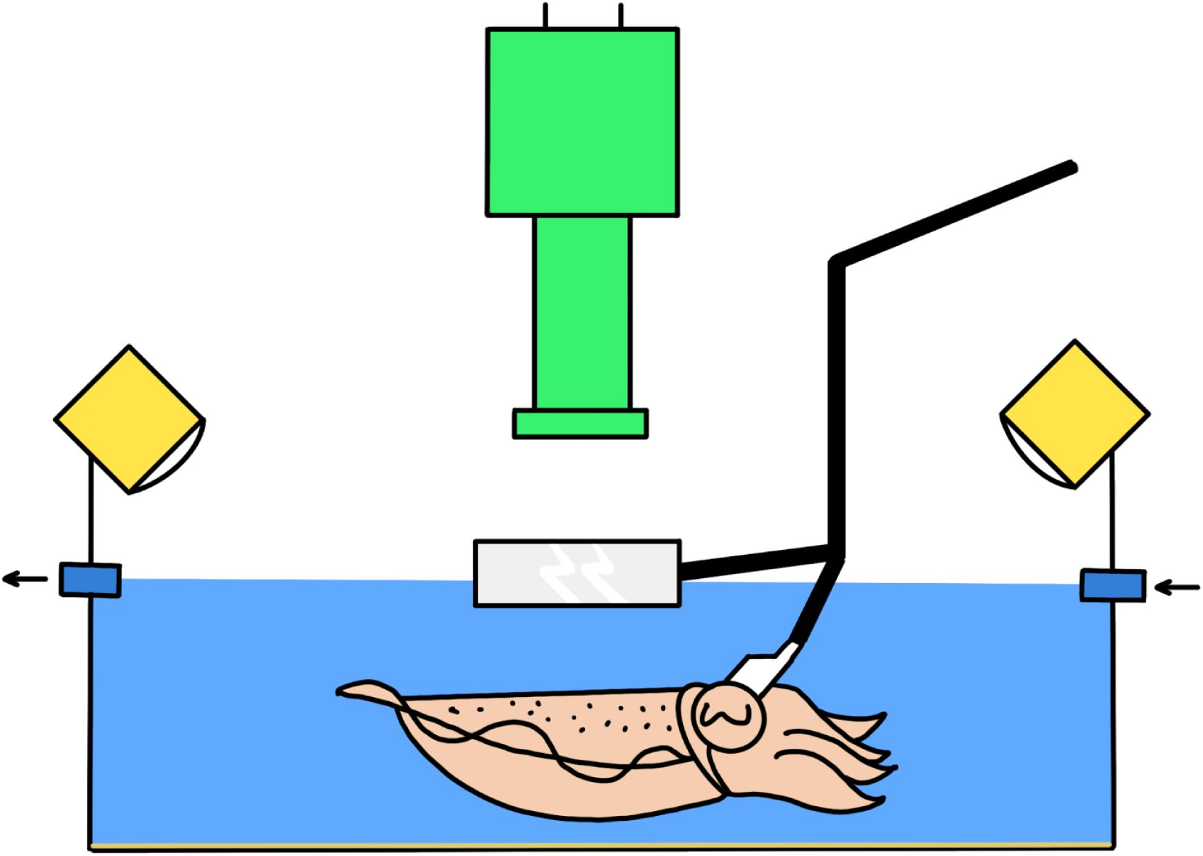
Schematics of experimental setup with head fixation.
The camera (green) is positioned above the tank, which is filled with artificial seawater (blue). A constant flow of water (indicated by arrows) ensures proper oxygenation. LEDs (yellow) surrounding the tank provide uniform illumination. A bracket (black) supports a thick glass panel (gray) to minimize water distortion during filming. The same bracket also holds a head-fixation mount (white) to stabilize the animal’s head.
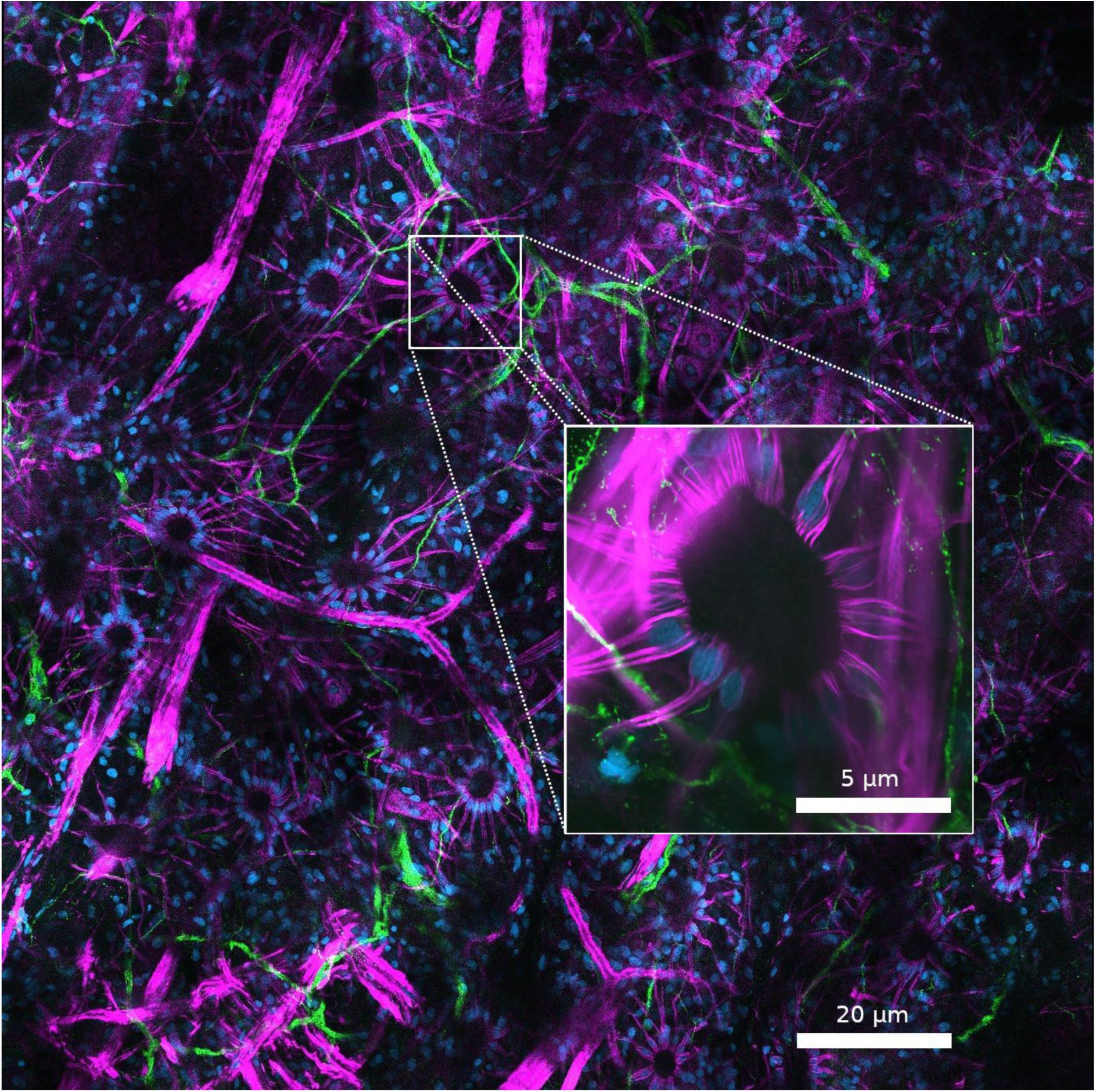
Confocal image of E. berryi’s stained skin captured with ZEISS LSM 980.
DAPI in blue (nuclei), phalloidin in magenta (muscle fibers), and tubulin in green (nerve fibers). A single chromatophore is highlighted (white box) to illustrate its cellular organization. Radial muscle fibers (magenta) extend outward from the central pigment sacculus, with nuclei (blue) arranged in a rosette at the base of each fiber. Tubulin-labeled nerve fibers (green) approach the muscles, suggesting potential neuromuscular connections, though the precise contact points cannot be confirmed in the absence of a neuromuscular junction marker.


