Quantification of gait parameters in freely walking wild type and sensory deprived Drosophila melanogaster
Figures
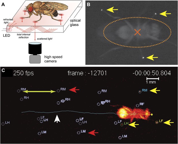
fTIR apparatus and FlyWalker software.
(A). Schematic of the fTIR optical effect. LED light sources are located at the edges of an optical glass and light propagates within the glass via internal reflection. Tarsal contacts lead to light scattering detected by a high-speed camera. See Figure 1—figure supplement 1 for more details. (B). Single frame of a fTIR video. The fTIR effect can be seen for three legs in stance phase (yellow arrows). Background light partially illuminates the fly's body (orange dashed ellipse; the center of the body is indicated by an orange cross). (C). Image generated by the FlyWalker software. The fly's footprints and body center are tracked throughout the video. Present footprints are identified and labeled (yellow arrows). The fly body and trajectory are visualized by a blue line (white arrow). Past footprints can also be recorded (red arrows). A scale bar can be introduced. Step length is defined as the distance between two consecutive footprints (green arrows).
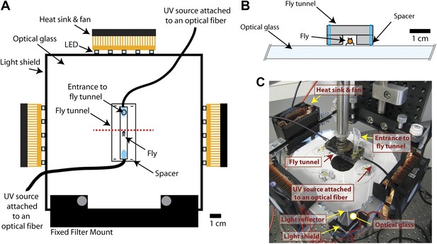
Additional information on fTIR apparatus.
(A). Detailed schematic of the fTIR apparatus. Red dashed line shows position of the cross-section image in panel (B). (B) Cross-section of schematic at red dashed line in panel (A). (C) Photograph of the fTIR apparatus.
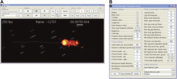
FlyWalker program.
(A). Screenshot of the FlyWalker graphical user interface used to edit fTIR videos. (B). Screenshot of the FlyWalker parameters window.
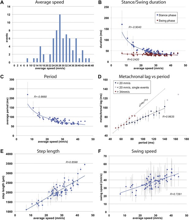
General walking parameters.
(A). Speed histogram of 71 videos recorded for wild type flies, with 2 mm/s bins. Average speeds vary between 7.2 and 44.7 mm/s, with 28 mm/s the most represented speed. Speeds at ∼20 mm/s are underrepresented in this dataset. (B). Durations of stance (blue) and swing (red) phases as a function of speed. Swing phase duration remains mostly constant while stance phase duration is inversely proportional to speed. Graphical fits for swing and stance phases versus speed are represented in red and blue lines, respectively. (C). Step period is inversely proportional to average speed. The blue line is a graphical fit. (D). Duration of the metachronal lag as a function of the hindleg period for slow (blue) and fast (red) flies. metachronal lag closely matches hindleg period for fast flies (HLagF ≈ Period). Regression line for the slow walking flies: HLagF = Period × 0.505 + 27.627. A total of 220 metachronal waves were used, error bars correspond the standard error of the mean. (E),(F). Step length (E) and swing speed (F) increase linearly with speed. A graphical fit is shown by the blue lines. Error bars in (B–F) correspond to standard error of the mean.
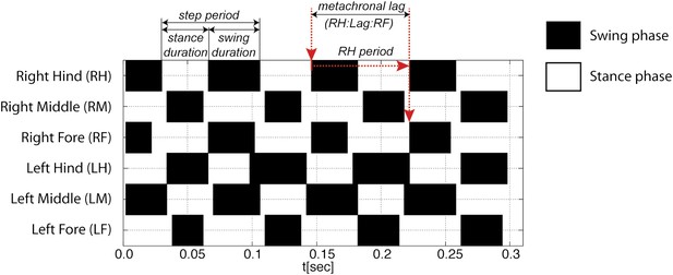
Gait definitions.
For each leg, swing phases are represented in black and stance phases are represented in white (from top to bottom: right hind (RH); right mid (RM); right front (RF); left hind (LH); left middle (LM); left front (LF)). Step period is the time for one complete cycle (initiation of consecutive stance phases) and is divided into stance duration and swing duration. The metachronal lag is defined as the time between the start of sequential swing phases for the hind and forelegs on the ipsilateral side (red arrows).
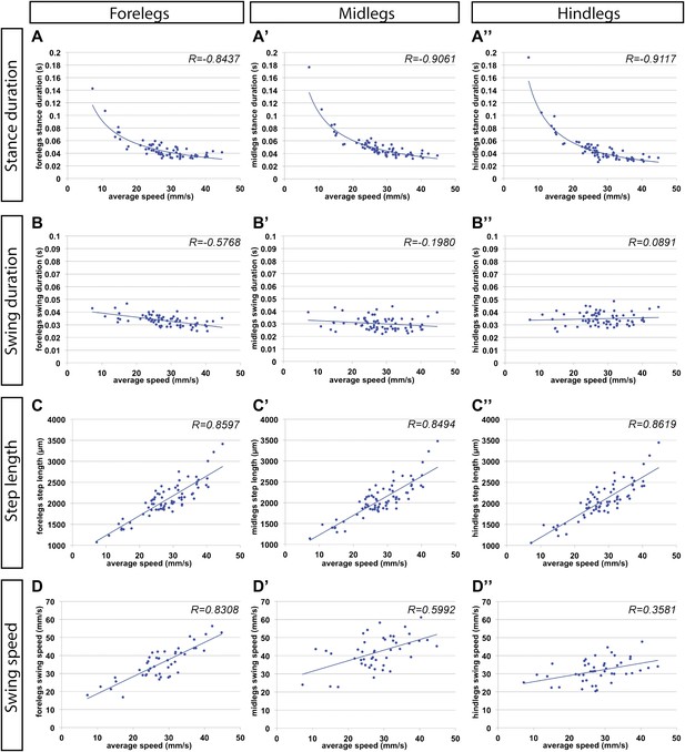
Gait parameters by segment.
(A)–(D). Each column corresponds to the legs in a particular segment. Graphical fits are represented by blue lines. (A) Stance duration. (B) Swing duration. (C) Step length. (D) Swing speed.
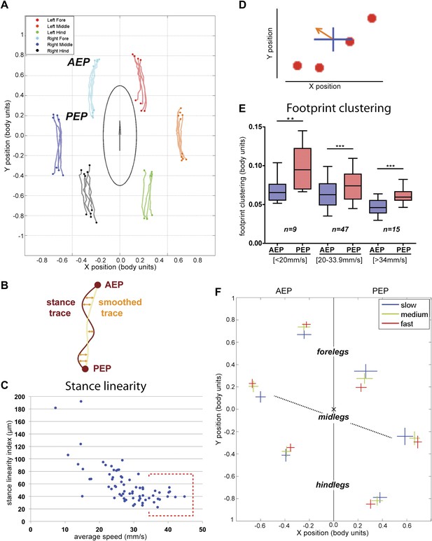
Spatial parameters.
(A). Stance traces. Representative plot of an animal walking at 28.82 mm/s. Traces are generated by the position of the stance phase footprints relative to the body center (set at 0.0,0.0). For each leg, stance onset corresponds to the Anterior Extreme Position (AEP) while stance offset is termed Posterior Extreme Position (PEP). (B). Method to quantify the stance linearity index. For each stance trace (brown), a smoothed trace is generated (using data from every five frames; yellow trace), and the average of the difference between these two lines (orange arrows) corresponds to the stance linearity index. (C). Stance linearity as a function of speed. Each data point corresponds to the average of all traces for all six legs for a single video greater than ∼34 mm/s, stance linearity becomes constant (red box). (D). Method to quantify footprint clustering. For each set of AEP/PEP footprints (red circles), an average ±STD xy point is created (blue cross). The footprint clustering value is calculated as the vector sum of the two STD values (orange arrow). (E). Quantification of footprint clustering. Data were grouped into slow (<20 mm/s), medium (between 20 and 34 mm/s) and fast (>34 mm/s) speeds. Boxplots represent the median as the middle line, with the lower and upper edges of the boxes representing the 25% and 75% quartiles, respectively; the whiskers represent the range of the full data set. Values are normalized for body size. Asterisks indicate the significance of the decrease in footprint clustering between the AEP and the PEP (using the paired parametric t test in the case of the slow speed group and the Wilcoxon non-parametric test for the remaining groups, **p<0.005, ***p<0.001). A comparison between the three speed groups also displays statistical significance (Kruskal–Wallis-ANOVA, p values of 0.0015 and 0.0014 for AEP and PEP, respectively). Dunn's post hoc significance tests show: slow AEP vs medium AEP, not significant (NS); medium AEP vs fast AEP, **; slow AEP vs fast AEP, **; slow PEP vs medium PEP, NS; medium PEP vs fast PEP, NS; slow PEP vs fast PEP, ***. (F). Footprint position relative to the body center. Data were pooled as in the previous panel. AEP and PEP values for each leg are represented on the left and right sections of the plot, respectively. Values are normalized for body size.
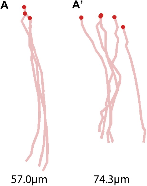
Representative examples of stance traces and corresponding stance linearity values.
A less linear stance trace (e.g., (A′) compared to (A)) corresponds a higher stance linearity value.
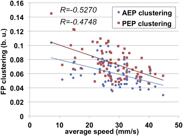
AEP and PEP clustering values for all segments as a function of speed.
Linear trend lines for AEP and PEP versus average speed are shown as blue and red lines, respectively.
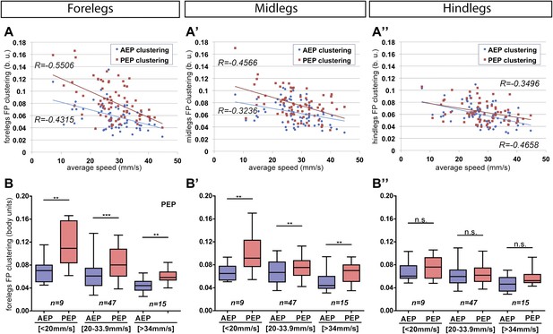
AEP and PEP clustering values for each segment as a function of speed.
(A). Linear trend lines for AEP and PEP are represented as blue and red lines, respectively. (A) forelegs; (A′) midlegs; (A″) hindlegs. (B). Boxplots of the data presented in (A). Data were grouped into slow (<20 mm/s), medium (between 20 and 34 mm/s) and fast (>34 mm/s) animals. Boxplots represent the median as the middle line, with the lower and upper edges of the boxes representing the 25% and 75% quartiles, respectively, and the whiskers representing the range of the full data set. Values are normalized for body size. Asterisks indicate statistical significance between AEP and PEP. (Data analyzed by the Wilcoxon or paired-t test the, **p<0.005, ***p<0.001). Values are normalized for body size.
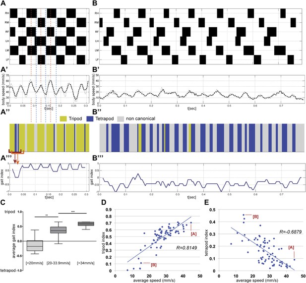
Gait parameters.
(A),(B). Upper panels show the step pattern for representative videos of animals walking at 44.7 (A) and at 14.6 mm/s (B). For each leg swing phases are represented in black (from top to bottom: right hind (RH); right mid (RM); right front (RF); left hind (LH); left middle (LM); left front (LF)). (A′),(B′) show the instantaneous speed for the same video. Thick and thin lines correspond to integration times of 25 or 12.5 ms, respectively. In faster animals (A), peak speeds are observed halfway through the stance phase (red dashed line), while minimum speeds are observed during gait transitions (blue dashed line). (A″),(B″), for each frame the corresponding gait was color coded as follows: green (tripod), blue (tetrapod), and gray (non-canonical). Red brackets indicate the eight frame windows used to generate the gait index plots (A‴),(B‴). Tripod = +1; tetrapod = −1; and noncanonical = 0. (C). Quantification of the average gait index for three speed groups. For each video the average gait index was calculated for all frames (p<0.0001 for Kruskal–Wallis-ANOVA test. Dunn's post hoc significance test: **p<0.005, ***p<0.001). (D),(E). Tripod (D) and tetrapod (E) indexes as a function of speed. Graphical fits are represented in blue. Data for points labeled (A) and (B) are shown in panels (A) and (B), respectively.
Gait features.
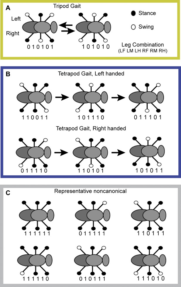
(A)–(C). Walking gaits and leg combinations. Each leg can be either in a swing or stance phase, represented by white or black circles, respectively. Underneath each combination the corresponding numerical code (‘1’ and ‘0’ correspond to stance or swing, respectively. Digit order: left foreleg; left midleg; left hindleg; right foreleg; right midleg; right hindleg. (A) Tripod gait combinations. (B) Tetrapod gait combinations. Tetrapod gait can be either right or left handed depending on which side is swinging more anteriorly. (C) Representative noncanonical combinations, which are not represented by tripod or tetrapod configurations.
Gait index plot.
(A). Average gait index as a function of speed. Each point corresponds to the average of all frames in a video (Figure 4A‴,B‴). (B). Instantaneous speed, gait map and gait index plots for data points labeled in (A) by I., II., and III. are shown. Data for points labeled A* and B* are shown in Figure 4A,B, respectively.
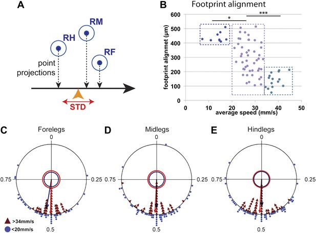
Coordination parameters.
(A). Method to calculate footprint alignment. For each set of footprints, the projection points along the displacement axis (horizontal black arrow) are calculated. Footprint alignment corresponds to the standard deviation (STD) of the average point (orange arrowhead). (B). Quantification of footprint alignment versus speed. Values are color coded according to speed group: <20 mm/s in dark blue; between 20 and 34 mm/s in purple and >34 mm/s in turquoise. Values cluster into three main groups indicated by the dotted boxes (p<0.0001 for Kruskal–Wallis-ANOVA test. Dunn's post hoc significance test: *p<0.005, ***p<0.001). (C)–(E). Radial plots of contralateral leg phases comparing slow (blue triangles) and fast (red triangles) walking animals. Mean r vectors for slow and fast animals are represented by blue and red arrows, respectively. Inner circles indicate a Rayleigh p value of 0.05.
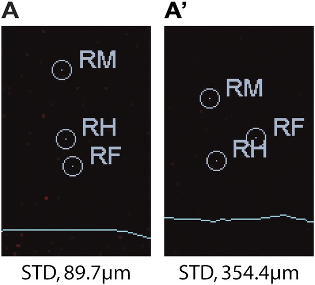
Representative images of footprints with different footprint alignment values.
https://doi.org/10.7554/eLife.00231.020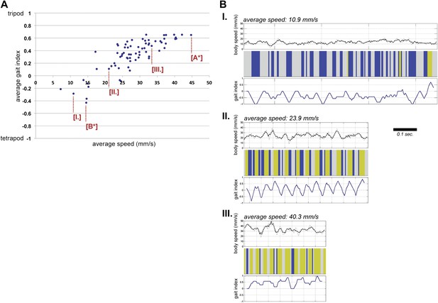
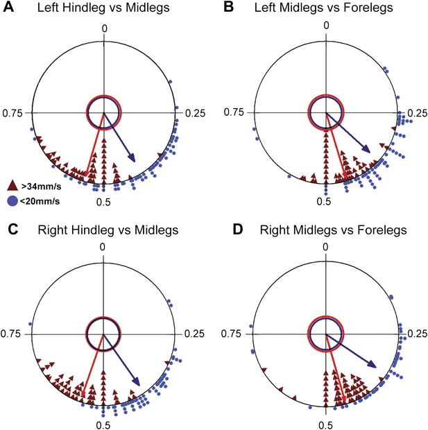
Radial plots of adjacent ipsilateral leg phases comparing slow and fast walking animals.
Individual data points for slow and fast flies are represented by blue circles and red triangles, respectively. Mean r vectors for slow and fast animals are represented by blue and red arrows, respectively. Inner circles indicate a Rayleigh p value of 0.05.
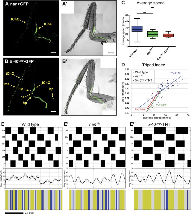
Effects of sensory deprivation on walking.
(A). Expression pattern driven by nanchung-Gal4. Genotype: F-Gal4, UAS-GFP. (B). GFP expression under combinatorial control of 5-40-Gal4 and dacRE-flp. Genotype: 5-40-Gal4, dacRE-flp, UAS-FRT-stop-FRP-GFP. All classes of sensory neurons in the leg express GFP. tChO, tibia chordotonal organ; fChO, femur chordotonal organ; hp, hair plates; cs, campaniform sensilla; ms, mechanosensory brisles. Bar, 100 μm. (C). Average speed. Boxplots with the median as the middle line and the lower and upper edges of the boxes representing the 25% and 75% quartiles, respectively; the whiskers represent the range of the full data set. Statistical analysis with one-way-ANOVA (p<0.0001) followed by Tukey's post hoc test, ***p<0.001. (D). Tripod index. Lines represent graphical fits. See Table 2 for statistical analysis. (E). Gait patterns, instantaneous speeds, and gait maps for representative wild type and sensory deprived animals walking at similar speeds. See Figure 2—figure supplement 1 for details. Tripod gait properties remain unchanged.
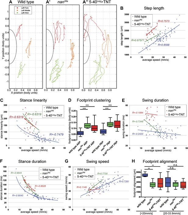
Quantification of gait parameters in sensory deprived animals.
(A). Stance traces of three representative animals walking at a similar speed. For simplicity, only left stance traces are shown. Traces for sensory deprived genotypes display a longer step length; higher jitter and a more variable AEP and PEP. (See panels (B)–(D) and (H) for quantification). In (B),(C) and (E)–(G), colored lines represent graphical fits. See Table 2 for statistical analysis of (B),(C),(E),(F) and (G). (B). Step length. Sensory deprived animals display an increased step length. (C). Stance linearity. Sensory deprived animals display a more jittery movement. (D). AEP and PEP footprint clustering. Wild type data correspond to the speed range of nan36a and 5-40Leg>TNT (12.6 to 27.7 mm/s). In (D),(H), boxplots represent the median as the middle line and the lower and upper edges of the boxes representing the 25% and 75% quartiles, respectively; the whiskers represent the range of the full data set. Statistical analysis with Kruskal–Wallis-ANOVA (p<0.0001) followed by Dunn's post hoc test, ***p<0.001. (E). Swing duration. (F). Stance duration. (G). Swing speed. (H). Footprint alignment. Slow-walking sensory deprived animals display more aligned footprints compared to wild type flies. Data were grouped into slow (<20 mm/s) and medium speeds (between 20 and 34 mm/s). Kruskal–Wallis-ANOVA test: p=0.0003 and NS for the slow and medium speed groups, respectively. Asterisks indicate the significance of the decrease in footprint clustering between genotypes. (Data analyzed by the Dunn's post hoc significance test, **p<0.005).
Videos
Unprocessed fTIR video.
Processed video by FlyWalker.
Processed video of 5-40Leg>TNT fly.
Tables
Gait combinations in three speed classesa
| Slow [≤19.9 mm/s] | Medium [20–33.9 mm/s] | Fast [≥34 mm/s] | |||
| Tripod | 31.37 | Tripod | 51.63 | Tripod | 64.98 |
| Tetrapod | 25.45 | Tetrapod | 15.90 | Tetrapod | 7.26 |
| Total | 56.82 | Total | 67.54 | Total | 72.24 |
| Additional combinations | Additional combinations | Additional combinations | |||
| 111110 | 8.27 | 111111 | 4.76 | 111011 | 4.89 |
| 110111 | 7.60 | 111110 | 4.61 | 111111 | 4.25 |
| 111111 | 6.38 | 011111 | 4.30 | 011111 | 4.07 |
| 111011 | 5.62 | 111011 | 4.26 | 010111 | 3.36 |
| 011111 | 5.03 | 010111 | 3.84 | 111010 | 2.80 |
| 010111 | 2.47 | 110111 | 3.79 | 110111 | 2.32 |
| 111010 | 2.45 | 111010 | 2.91 | 111110 | 1.29 |
| 101111 | 1.94 | 101111 | 0.71 | 011011 | 1.25 |
| 111101 | 1.69 | 011011 | 0.52 | 011010 | 0.69 |
| Pentapod | 30.15 | Pentapod | 14.37 | Pentapod | 13.33 |
| 3 gaits combinedb | 86.97 | 3 gaits combinedb | 81.91 | 3 gaits combinedb | 85.57 |
| Totalc | 98.3 | Totalc | 97.2 | Totalc | 97.15 |
-
a
Values are expressed as percentage (%). Leg order in combination: LF LM LH RF RM RH. 1, footprint present; 0, footprint is absent.
-
b
The sum of tripod, tetrapod, and pentapod gaits.
-
c
The sum of all gait patterns listed in the table.
Multiple regression models for wild type versus sensory-deprived fliesa
| Wild type vs nan36a | |||||||||||||||||||
| Step length (Figure 7B) | Stance linearity (Figure 7C) | Swing duration (Figure 7E) | Swing speed (Figure 7G) | Stance duration (Figure 7F) | Tripod index (Figure 6D) | ||||||||||||||
| Coef | SE | p-value | Coef | SE | p-value | Coef | SE | p-value | Coef | SE | p-value | Coef | SE | p-value | Coef | SE | p-value | ||
| WT y intercept | 746.7 | 93.8 | 0.0 | 291.6 | 32.6 | 0.0 | 3.6 × 10⁻² | 1.9 × 10⁻³ | 0.0 | 19.1 | 2.1 | 0.0 | 2.3 × 10⁻¹ | 1.2 × 10⁻² | 0.0 | −9.2 × 10⁻⁴ | 4.2 × 10⁻² | 0.982 | |
| Δ y intercept | 587.4 | 270.5 | 0.0 | 349.8 | 96.4 | 0.0 | 2.2 × 10⁻² | 5.2 × 10⁻³ | 0.0 | −4.5 | 5.9 | 0.451 | 1.9 × 10⁻¹ | 3.4 × 10⁻² | 0.0 | −4.1 × 10⁻¹ | 1.2 × 10⁻¹ | 0.001 | |
| WT slope | 47.2 | 3.3 | 0.0 | −70.9 | 9.9 | 0.0 | −1.3 × 10⁻⁴ | 6.4 × 10⁻⁵ | 0.043 | 0.6 | 0.1 | 0.0 | −5.4 × 10⁻² | 3.5 × 10⁻³ | 0.0 | 1.8 × 10⁻² | 1.4 × 10⁻³ | 0.0 | |
| Δ Slope | −11.3 | 12.9 | 0.4 | −89.1 | 32.1 | 0.007 | −8.4 × 10⁻⁴ | 2.5 × 10⁻⁴ | 0.001 | 0.5 | 0.3 | 0.115 | −1.6 × 10⁻² | 4.8 × 10⁻³ | 0.002 | 1.6 × 10⁻² | 5.6 × 10⁻³ | 0.006 | |
| Wild type versus 5-40Leg>TNT | |||||||||||||||||||
| WT y intercept | 746.7 | 93.8 | 0.0 | 291.6 | 34.0 | 0.0 | 3.6 × 10⁻² | 1.9 × 10⁻³ | <0.001 | 19.1 | 2.1 | <0.001 | 2.3 × 10⁻¹ | 1.2 × 10⁻² | 0.0 | −9.2 × 10⁻⁴ | 4.3 × 10⁻² | 0.983 | |
| Δ y intercept | 622.8 | 295.3 | 0.038 | 242.2 | 115.7 | 0.039 | 1.7 × 10⁻² | 1.0 × 10⁻³ | <0.001 | 10.5 | 6.4 | 0.1 | 1.6 × 10⁻¹ | 4.1 × 10⁻² | 0.0 | −3.6 × 10⁻¹ | 1.4 × 10⁻¹ | 0.009 | |
| WT slope | 47.2 | 3.2 | 0.0 | −70.9 | 10.3 | 0.0 | −1.0 × 10⁻⁴ | 6.0 × 10⁻⁵ | 0.04 | 0.7 | 0.1 | <0.001 | −5.4 × 10⁻² | 3.7 × 10⁻³ | 0.0 | 1.8 × 10⁻² | 1.5 × 10⁻³ | 0.0 | |
| Δ Slope | 11.4 | 15.6 | 0.465 | −54.8 | 39.7 | 0.17 | −2.4 × 10⁻⁵ | 3.1 × 10⁻⁴ | 0.94 | −0.5 | 0.3 | 0.12 | −4.4 × 10⁻² | 1.4 × 10⁻² | 0.003 | 1.6 × 10⁻² | 7.1 × 10⁻³ | 0.032 | |
-
a
Coef stands for the estimated regression coefficient, SE represents its standard error. In this model we log transformed average speed for parameters that were non-linear with respect to speed (step linearity and stance duration). WT y intercept indicates the y intercept for wild type. Δ y intercept indicates the difference in the y intercept between the experimental condition and wild type. WT slope reports the slopes of the wild type regression lines. p-values >0.05 are in bold italics; those <0.05 are in italics underlined. If Δ slope is >0.05 (bold italics) the regression curves are considered non-interacting (∼parallel). If Δ y intercept is <0.05 (italics underlined), the parameter is considered different from WT.


