Modelling dynamics in protein crystal structures by ensemble refinement
- Utrecht University, The Netherlands
- Lawrence Berkeley National Laboratory, United States
- University of California Berkeley, United States
Figures
Figure 1
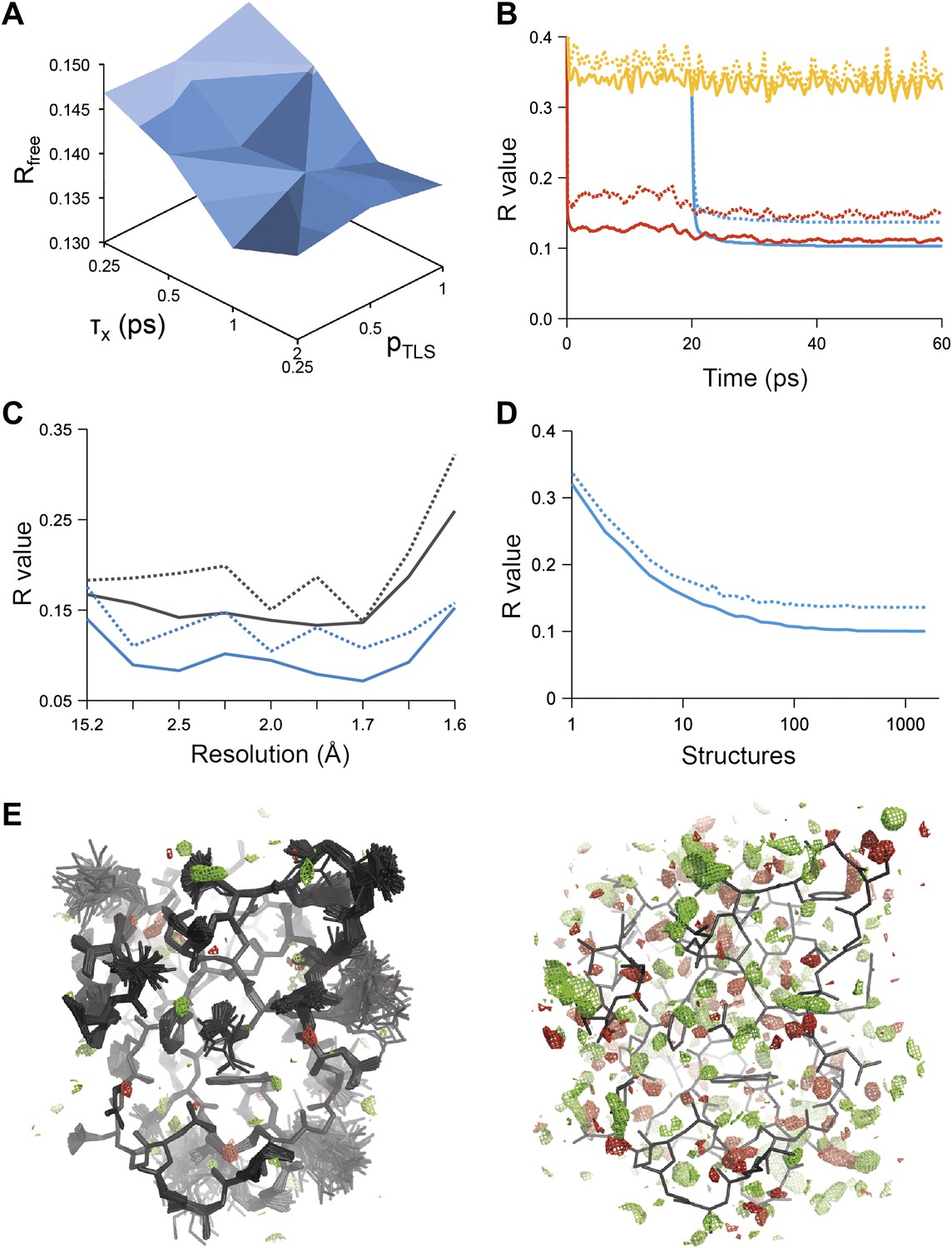
Example of ensemble refinement for dataset 1UOY. (A) Optimisation of empirical ensemble refinement parameters (τx, pTLS and Tbath). Simulations are performed independently and in parallel. The plot shows effect of τx, pTLS on Rfree (each grid point corresponds to the lowest Rfree among all Tbath values). Optimum parameters are selected by Rfree. (B) R-values obtained during ensemble-refinement simulation, solid lines Rwork and dashed lines Rfree; high values are observed for instantaneous models (yellow) contrasting with the rolling average used in the target function (red) and the final ensemble (blue). (C) R-values are reduced throughout the resolution range for ensemble model (blue) compared with phenix.refine re-refined single structure (black); solid lines Rwork and dashed line Rfree. (D) Number of structures in the ensemble, reduced by equidistant selection, versus Rwork (solid line) and Rfree (dashed line). Final number of structures is selected as the minimum number required reproducing the Rfree + 0.1%; in this case resulting in an ensemble containing 167 structures. (E) Density difference maps for the ensemble structure (mFobs − DFmodel)exp[iφmodel], left-hand side, and the single structure right-hand side, contoured at 0.34 e/Å3 (equivalent to 3.0 σ for the ensemble model), positive and negative densities are coloured green and red respectively. All molecular graphics figures are drawn using PyMol (The PyMOL Molecular Graphics System, Schrödinger, LLC).
Figure 2
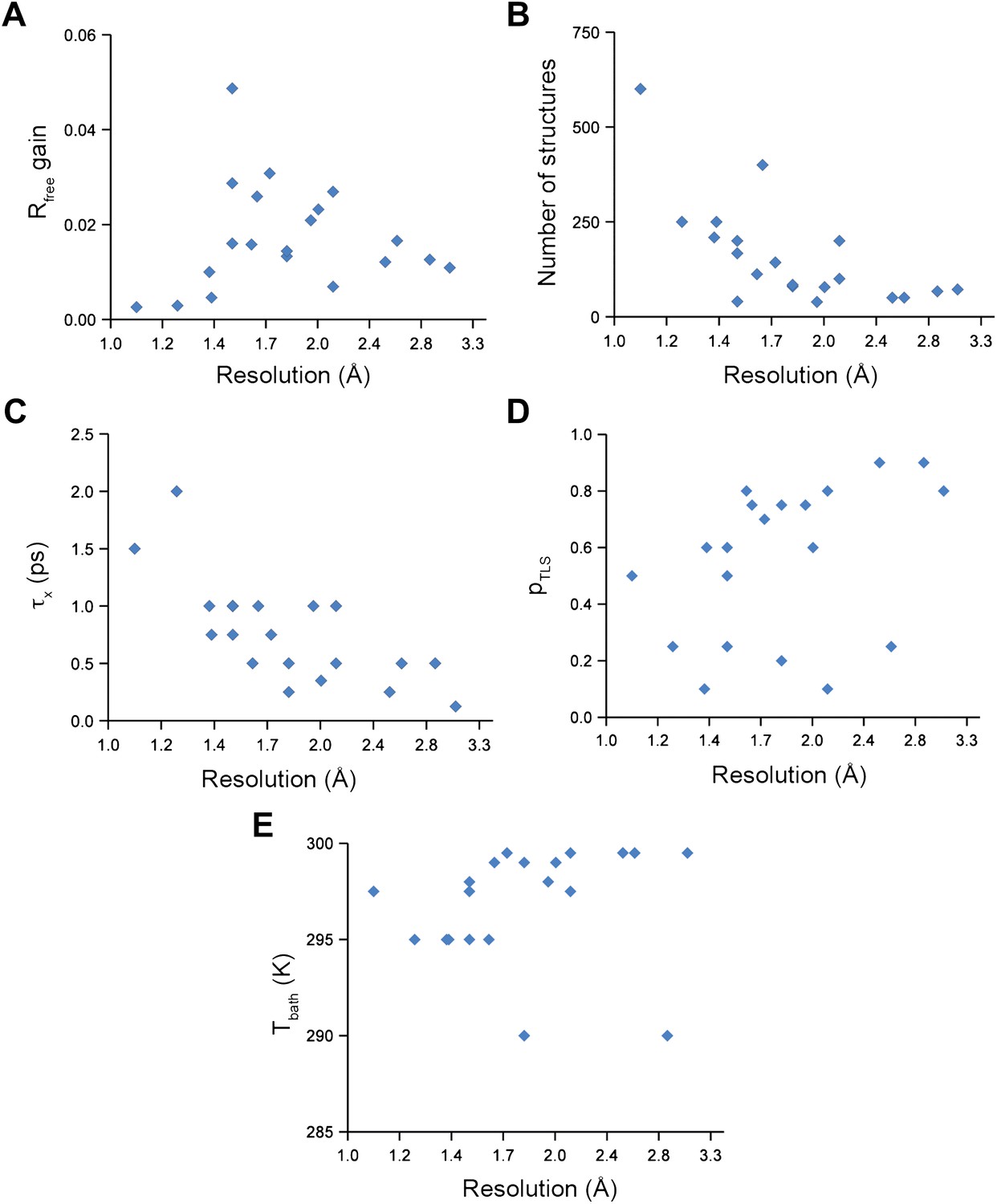
Ensemble refinement parameters and results as function of resolution of the datasets. (A) Gain in Rfree of ensemble refinement compared with re-refinement using phenix.refine, (B) number of structures in the final ensemble model, (C) optimum relaxation time, τx, (D) optimum pTLS and (E) optimum Tbath plotted as function of resolution of the dataset.
Figure 3
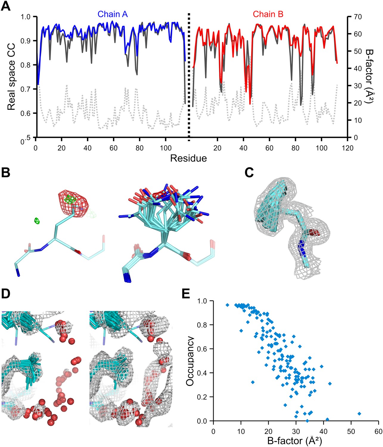
Validation of ensemble refinement using dataset 1YTT with exceptionally high quality experimental phases. (A) Real space cross-correlation of experimentally phased electron density map (|Fobs|exp[iφobs]) and model map (|Fmodel|exp[iφmodel]) for the single-structure (black) and ensemble model (chain A and B, blue and red respectively) shows improvements particularly for disordered areas (atomic B-factors from the re-refined single structure are shown in grey dashed lines). (B) Example of improved vector-difference map (|Fobs|exp[iφobs] − |Fmodel|exp[iφmodel]), contoured at 0.71 e/Å3 equivalent to 2.5 σ for the single structure for Gln167, chain A, for single (left-hand side) and ensemble structure (right-hand side). (C) Conformer distribution of Phe121 (chain A) with the experimental phased map (|Fobs|exp[iφobs]) contoured at 1.4 σ is highly similar to the multi-conformer shown in Figure 1c in Burling et al. (1996). (D) Partially disordered solvent shell (red) around residue Leu203 (chain A) as anticipated in Burling et al. (1996). Ensemble structure with experimental phased experimental map (|Fobs|exp[iφobs]) contoured at 1.4 σ (left side) and 0.7 σ (right side), as shown in Figure 2b in Burling et al. (1996). (E) Scatter plot showing the anti-correlation between the B-factor of explicit solvent molecules in the re-refined single-structure and the relative occupancy of water molecules at that same position (within 0.5-Å distance) in the ensemble model. Due to the difficulty in differentiating between disorder (B-factor) and occupancy for explicitly modelled water atoms in single structures a high B-factor is likely to correspond to a partially occupied site.
Figure 4
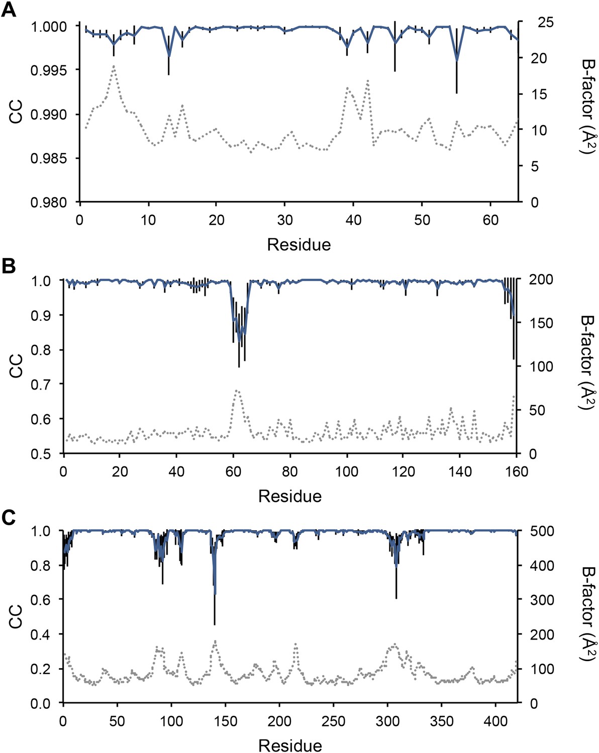
Sampling reproducibility of ensemble refinement. (A) Cross-correlations (CC) calculated for all pairs from 10 random-number seed repeat ensemble refinements of the 1UOY dataset extending to 1.5-Å resolution. (B) Cross correlations computed for 1BV1 (2.0-Å resolution); and, (C) for 3CM8 (2.9-Å resolution). Mean CC shown in solid blue (black error bars indicate ±1 σ). Cross correlations were computed from real-space Fmodel electron-density map correlations (Brändén and Jones, 1990). B-factors from the single structures refined using phenix.refine are shown in dotted grey lines.
Figure 5
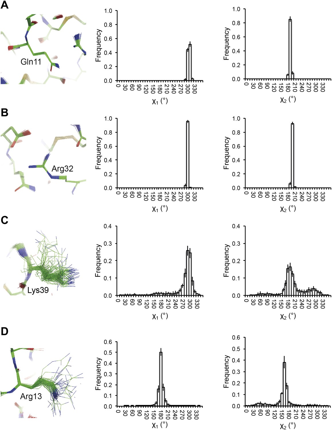
Reproducibility of side-chain rotamer distributions. Mean χ1 and χ2 distributions of four side-chains from the 10 repeats, with error bars ±1 σ, are shown for 1UOY. The four residues presented are those with the two highest CC values (see Figure 4A), (A) Gln11 (0.9999) and (B) Arg32 (0.9999), and the two lowest CC values, (C) Lys39 (0.9976) and (D) Arg13 (0.9966).
Figure 6
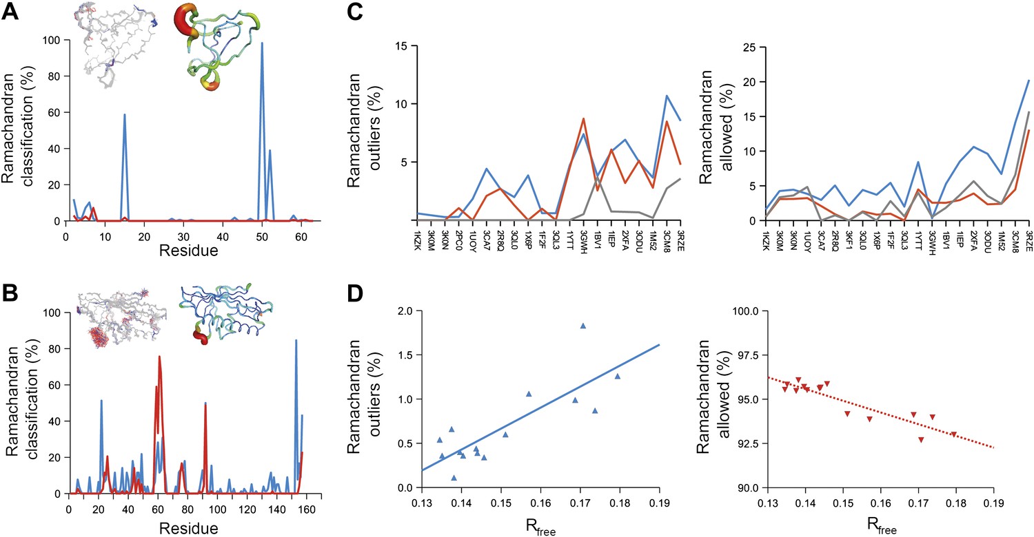
Ramachandran analysis. Distribution of Ramachandran torsion angles classified as outliers (red) and allowed (blue) for ensemble models, 1UOY (A) and 1BV1 (B). Plot shows percentage of classification per residue (i.e. relative number of times a φ,ψ-torsion angle combination is scored as outlier or allowed as defined by phenix.ramalyze). Structure inserts show (left-hand side) the location of the non-favourable torsion angles, outliers (red) and allowed (blue), and (right-hand side) a B-factor putty representation for the single structure refined with phenix.refine. (C) Overall Ramachandran statistics for ensemble and re-refined models. The Ramachandran statistics for the ensemble models are calculated in two ways: blue shows the percentage of outliers (left side) or allowed (right side) from all structures in the ensemble (cf. ‘whole distribution’ in Figure 6—source data 1), whereas red shows these percentages based on the most frequent occurring classification of each φ,ψ combination (cf. ‘centroid distribution’). The grey lines show the percentage of allowed (left side) and outliers (right side) for the re-refined single structures. Ramachandran statistics per re-refined single structure and ensemble are given in Figure 6—source data 2. (D) Correlation of Ramachandran statistics with Rfree values obtained from ensemble refinement. Three ensemble refinements were performed for the dataset 1UOY using different random-number seeds at Tbath values of 220, 260, 280, 290 and 295 K. Shown are the number of Ramachandran outliers (left side) and allowed (right side) in the ensemble as function of the Rfree value.
-
Figure 6—source data 1
Geometries of single-structure models and ensemble models.
Rms deviations (RMSD) from ideal bond, angle and dihedral geometries calculated for single structures re-refined using phenix.refine. Geometries for ensemble structures were calculated using two methods, the ‘whole distribution’, where the RMSD was calculated for each restraint (averaged over all structures), √〈(xideal − xmodel)2〉, and ‘centroid’ where the RMSD was calculated using the mean deviation from ideality for each restraint, √〈(〈xideal − xmodel〉)2〉, which for unimodal functions equals √〈(xideal − 〈xmodel〉)2〉.
- https://doi.org/10.7554/eLife.00311.013
-
Figure 6—source data 2
Ramachandran statistics for re-refined and ensemble models.
The Ramachandran statistics for the ensemble models are calculated in two ways: ‘Ramachandran (mean)’ shows the percentage of outliers, allowed and favoured averaged over all structures in the ensemble (cf. ‘whole distribution’ in Figure 6—source data 1), whereas ‘Ramachandran (mode)’ shows these percentages based on the most frequent occurring classification of each φ,ψ combination (cf. ‘centroid distribution’ in Figure 6—source data 1).
- https://doi.org/10.7554/eLife.00311.014
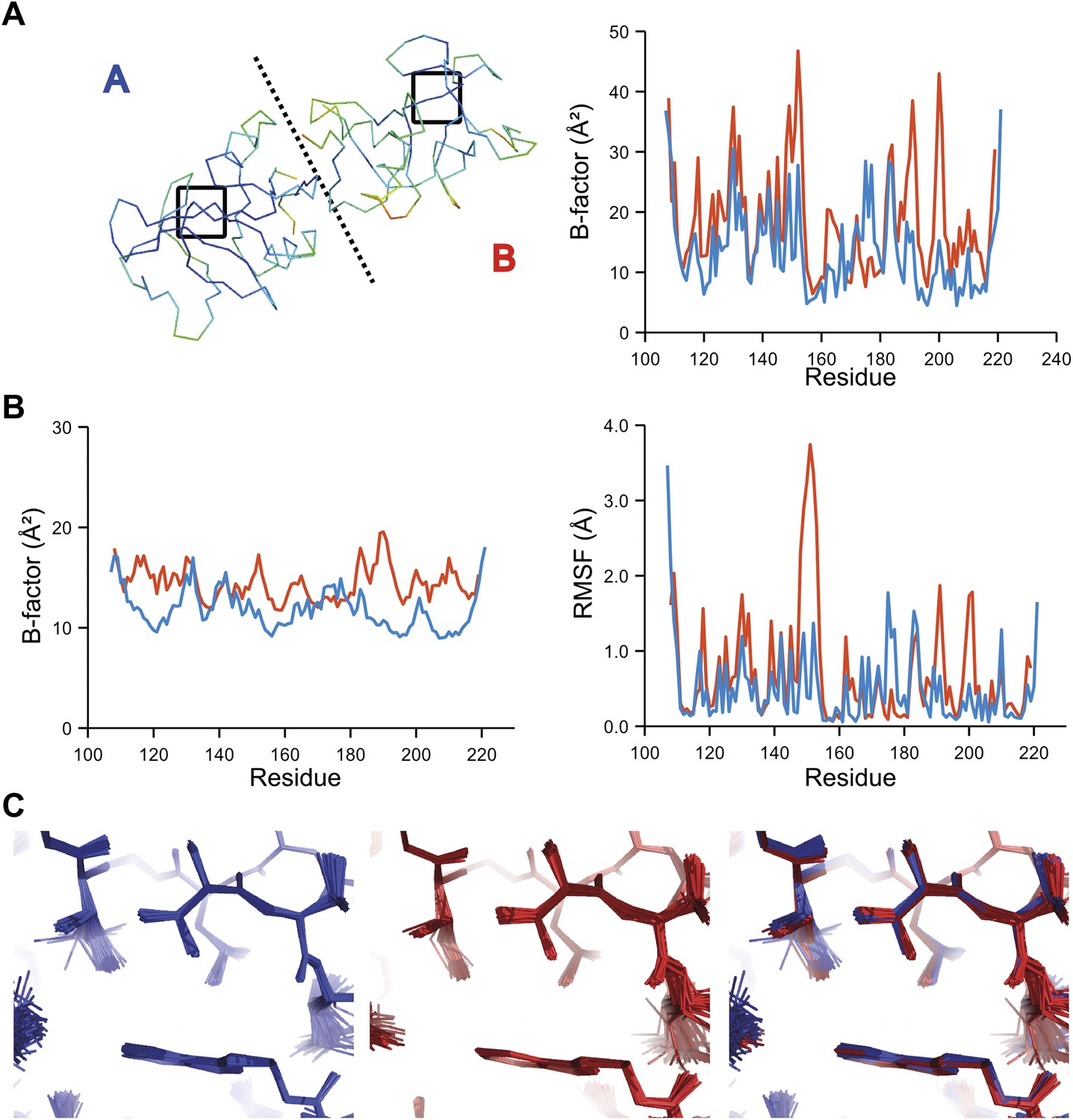
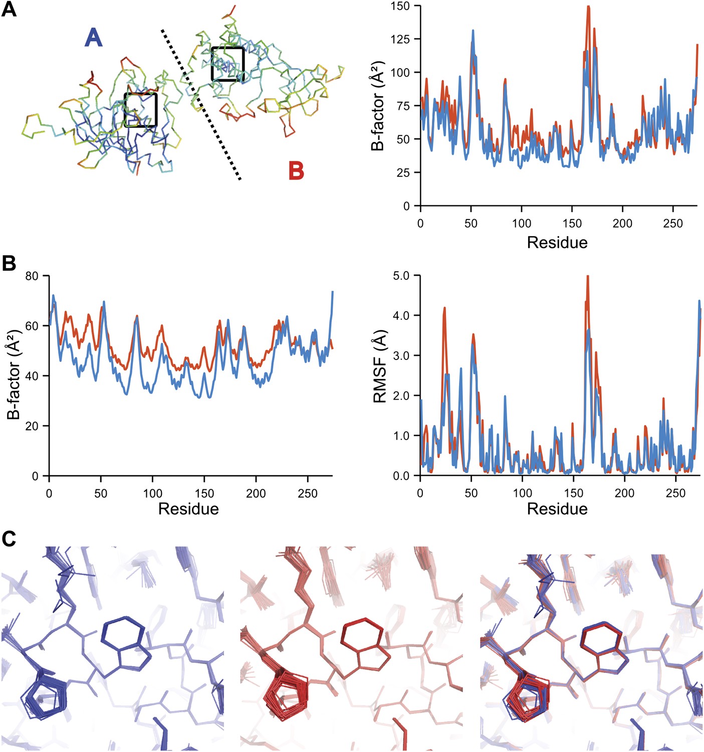
Figure 7 with 4 supplements
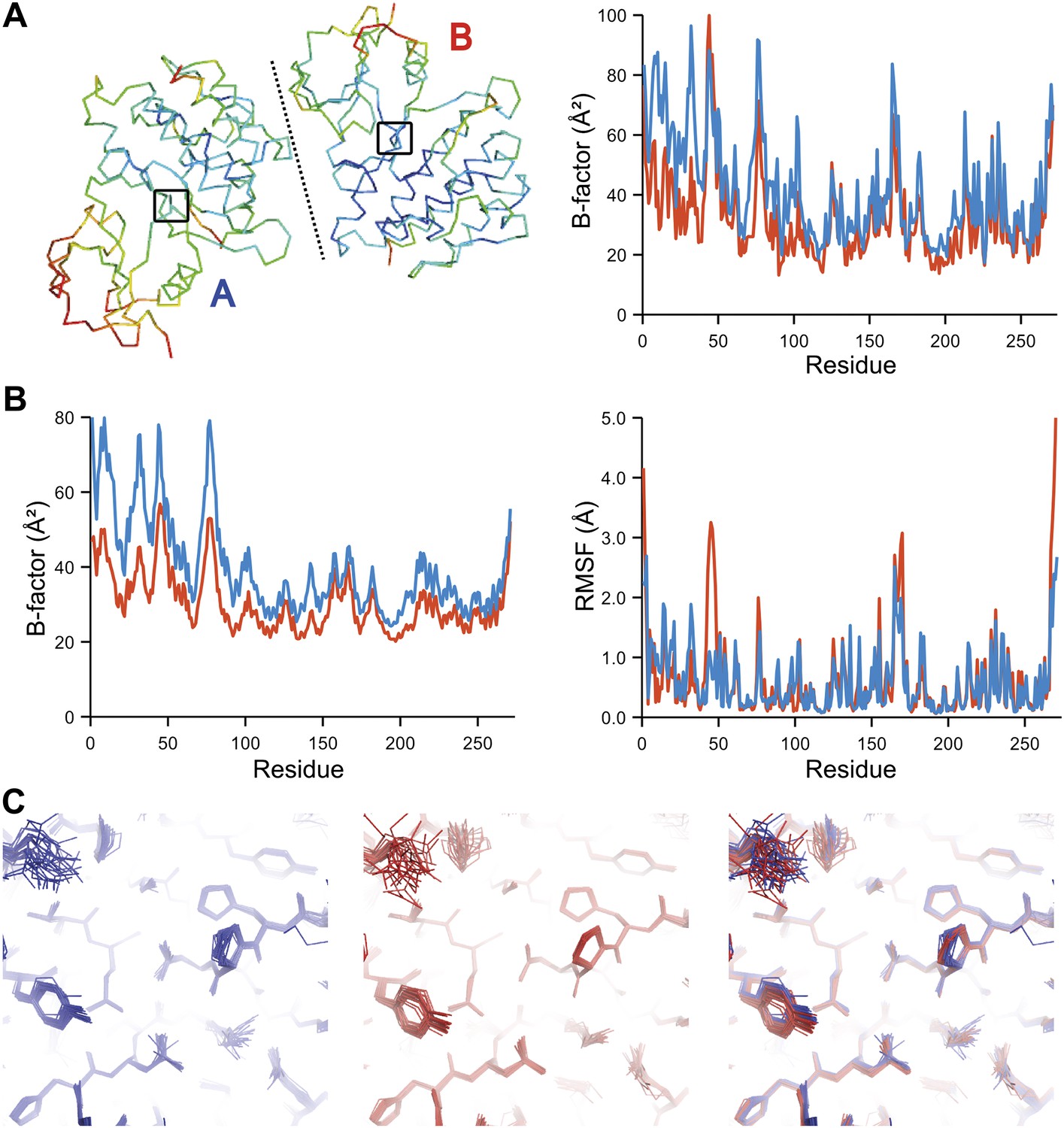
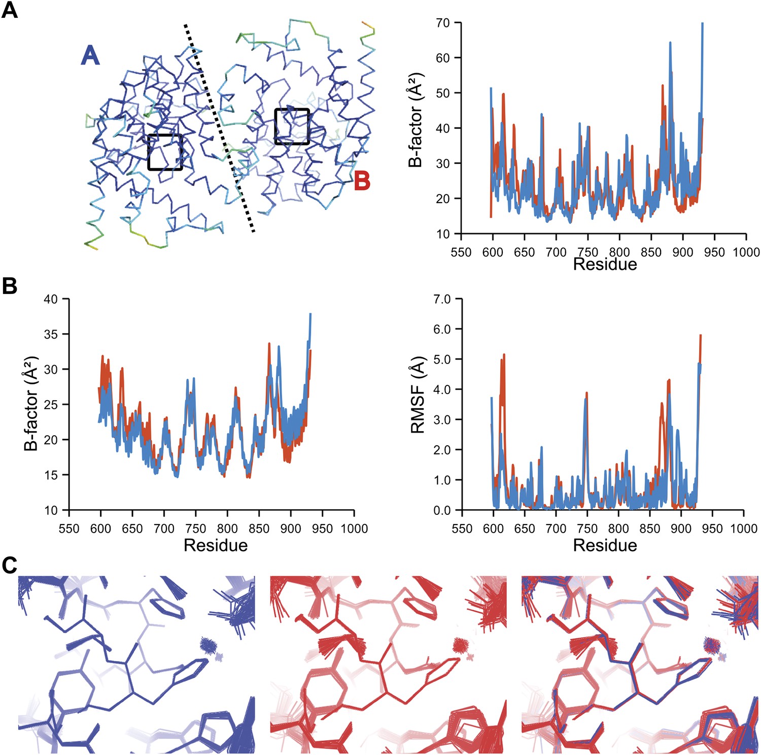
Comparison of atomic fluctuations for non-crystallographic symmetry related protein copies for dataset 1M52. (A) Cα trace of the re-refined single structure coloured by B-factor (from blue to red with increasing B-factor) for the two chains (left) and the B-factors plotted per residue number for protein chain A (blue) and B (red) (right). (B) B-factors from the basal TLS model (left) and rms atomic fluctuations (right) in the ensemble model averaged per residue. Differences in crystal packing restrict the flexibility of chain B around residue 47. (C) Comparison (left) and superposition (right) of a region of the protein (indicated by black box in (A)) of the ensemble of structures observed for protein copy A (blue) and B (red). Analogous analyses for 2R8Q, 1YTT, 1IEP and 2XFA are shown in Figure 7—figure supplements 1–4. The protein copies in 3GWH and 3ODU showed backbone shifts greater than 4.5 Å and were left out of this analysis.
Figure 7—figure supplement 1
Comparison of atomic fluctuations for NCS related protein copies for dataset 2R8Q.
Figure 7—figure supplement 2
Comparison of atomic fluctuations for NCS related protein copies for dataset 1YTT.
Figure 7—figure supplement 3
Comparison of atomic fluctuations for NCS related protein copies for dataset 1IEP.
Figure 7—figure supplement 4

Comparison of atomic fluctuations for NCS related protein copies for dataset 2XFA.
Figure 8
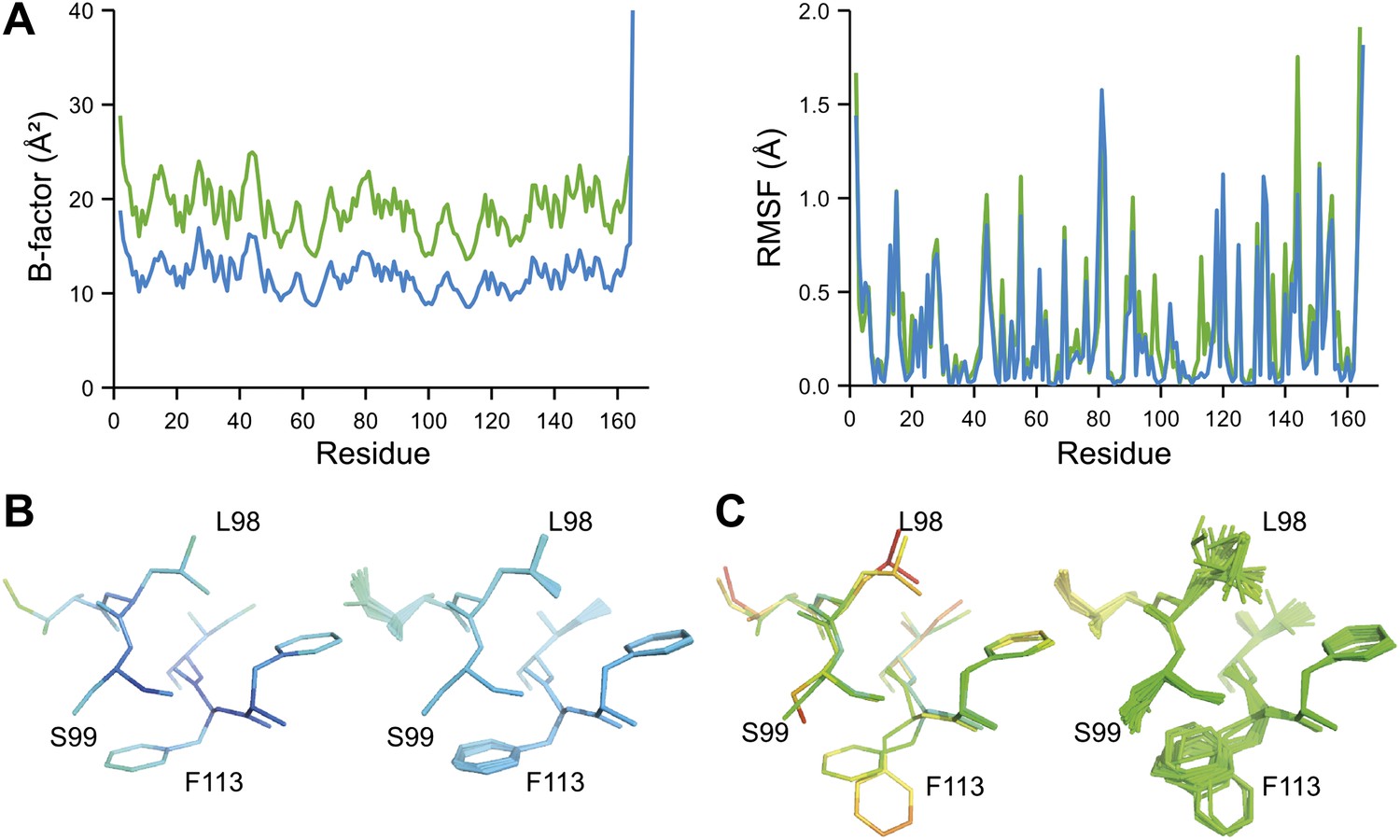
Ensemble refinement of two isomorphous proline isomerase datasets collected at 100 K and 288 K. (A) Left, basal TLS B-factors of ensemble models for 100 K and 288 K datasets (blue and green, respectively). Right, atomic rms fluctuations of ensemble models for 100 K and 288 K datasets (blue and green, respectively). (B) Re-refined single-structure (left) and ensemble model (right) for 100 K dataset. (C) Re-refined single-structure and ensemble model for 288 K dataset. In (B) and (C) atoms are coloured by B-factor (5 to 25 Å2). As with the published single structure refinement (Fraser et al., 2009) alternative conformations were not found for residues Leu98, Ser99 and Phe113 at 100K.
Figure 9

Overview of side-chain dynamics in ensemble structures. Atoms are coloured by their relative probability in the ensemble (see ‘Materials and methods’), reflecting the degree of disorder (ranging from well-ordered in blue to disordered in red). Bottom left insert shows secondary structure cartoon. Three datasets exhibit disordered interior sides chains forming a molten core region. (A) 3CA7 shows an ordered core with disordered hydrophilic side chains on the outside and is typical of the majority of the datasets. (B) 1BV1, the major pollen allergen and putative plant steroid transporter, has a disordered central cavity (location of cavity show with dotted lines). (C) 1X6P in the monomeric form of the fibril forming PAK pilin shows multiple disordered aliphatic and aromatic side chains in the interface between the N-terminal α-helix and the four stranded β-sheet domain. (D) Proline isomerase exhibits a molten core at 288 K, 3K0N (left); however, these interior dynamics are frozen-out at 100 K, 3K0M (right).
Figure 10
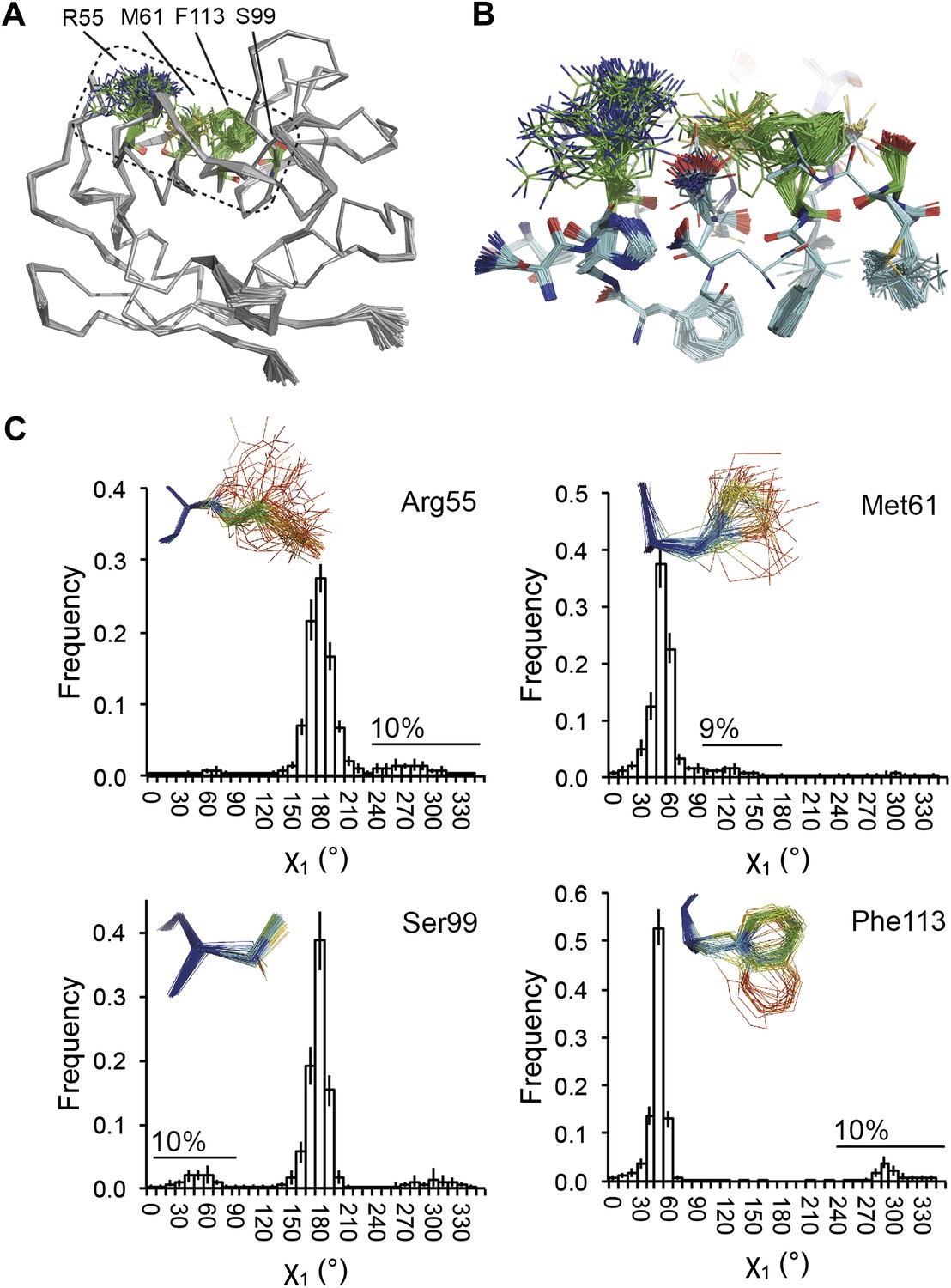
Dynamics in the binding pocket of proline isomerase at 288 K. (A) The location of the binding pocket comprised of residues Arg55, Met61, Ser99 and Phe113. (B) Zoom in of binding pocket (as dotted lines in (A)) showing flexible β-sheet for C=O·HN network of residues 55-62-113-98 in neighbouring β-strands. (C) All four residues show a ∼9:1 ratio between major and minor conformations which is in good agreement with NMR relaxation dispersion data collected a similar temperature (Eisenmesser et al., 2005). Histograms show mean χ1 angles generated from 10 random number repeats of ensemble refinement (error bars ±1 σ). Inserts show the relevant side chains, coloured by atomic probability (see ‘Materials and methods’), as observed in the ensemble reported in Table 1.
Figure 11
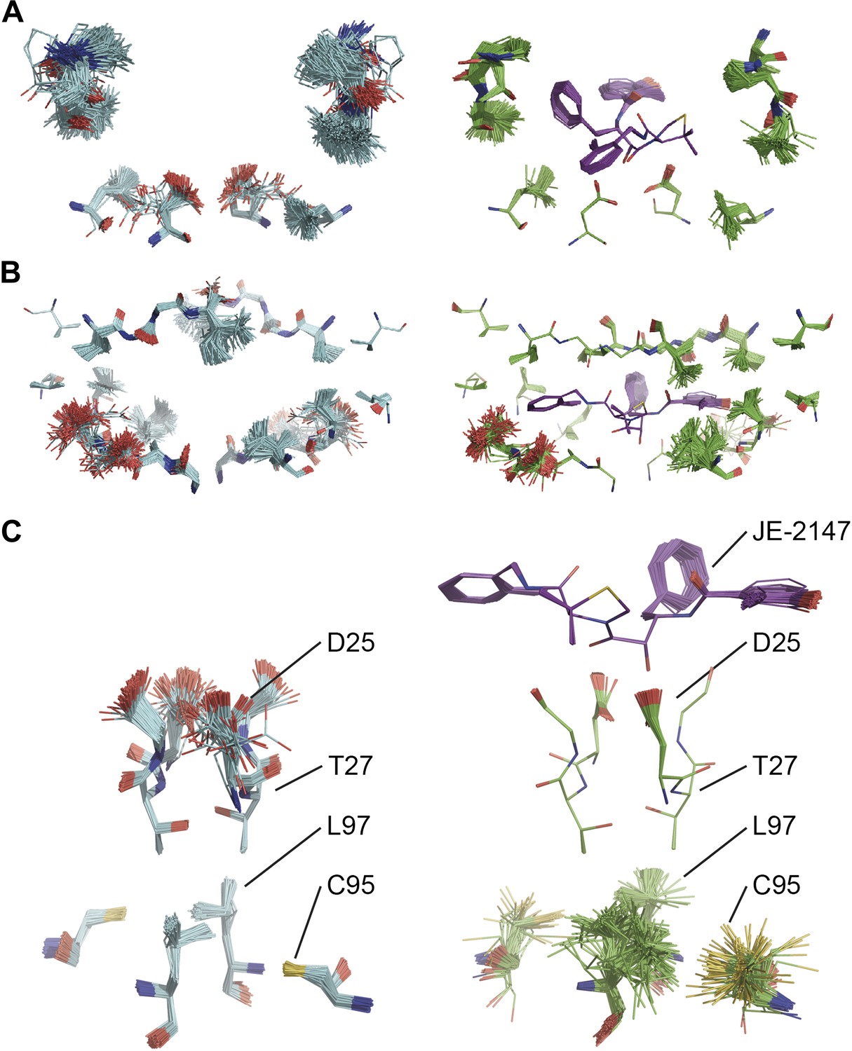
Comparison of ensemble structures of bound and unbound forms of HIV protease. (A) Residues in the P1 binding sites are disordered in the unbound HIV protease (2PC0), left-hand side, with carbon atoms shown in cyan, oxygen red and nitrogen blue. These residues become ordered in HIV protease in complex with a high affinity inhibitor, JE-2147 (1KZK), right-hand side with carbon atoms of the protease shown in green and of the inhibitor in purple. In 1KZK the two chains of the functional dimer are present in the asymmetric unit, whereas in 2PC0 a monomer is present in the asymmetric unit and the dimer is drawn using the crystallographic twofold axis. (B) Shows an alternative orientation showing the P2 binding site. (C) The catalytic Asp25 becomes ordered upon binding of the inhibitor, forming a hydrogen bond with the P1 carbonyl and hydroxyl of JE-2147. In contrast, the distal residues Cys95 and Leu97 at the dimer interface become less ordered upon binding.
Figure 12
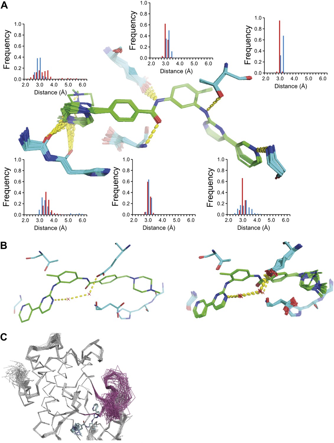
ABL-kinase Imatinib binding site. (A) Imatinib binding site in chain A of the 1IEP dataset showing distribution of the six protein–ligand hydrogen bonds in chain A and chain B (red and blue respectively). (B) Hydrogen bond network of ordered water network observed in the re-refined single structure, left, and the ensemble model, right. (C) The activation loop (shown in pink) is disordered when ABL-kinase is complexed with Imatinib (shown in cyan) as observed previously in solution (Vajpai et al., 2008).
Figure 13
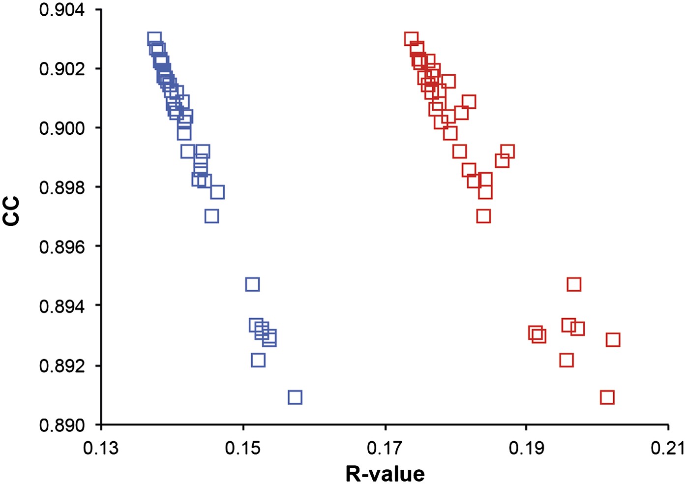
Correlation of R-values and overall map correlation coefficient for the 1YTT dataset in the block selection procedure. The correlation coefficients are calculated between the experimentally phased electron density map (|Fobs|exp[iφobs]) and ensemble model maps (|Fmodel|exp[iφmodel]) computed for different blocks of consecutive simulation times; blue squares indicate Rwork and red squares indicate Rfree.
Figure 14

Interpretation of global and local details of 1UOY ensemble model is aided by relative atomic probability (as described in ‘Materials and methods’). Ensemble models, left and centre, are colour by individual atom probability (0–1) from red to blue. Single structures, right, are coloured by individual atomic B-factor as refined in phenix.refine. (A) Global structure, selecting different probability ranges highlights partially ordered water positions. (B) Atomic probabilities of loop regain features correlate with B-factors in single structure. Anharmonic motion of Ser5 can be observed as well as anisotropic motion at Tyr7, which is shown in more detail in (C).
Tables
Table 1
Ensemble refinement statistics for 20 datasets. Datasets were taken from the PDB or PDB_REDO and were re-refined using ensemble refinement and phenix.refine. The relaxation time τx used, the resulting number of structures in the final ensemble and Rwork and Rfree values are given. The ensemble models yield improved Rfree values for all datasets, ranging in improvement from 0.3% to 4.9% with a mean improvement of 1.8%. The PDB accession numbers are as follows: 1KZK (Reiling et al., 2002), 3K0M (Fraser et al., 2009), 3K0N (Fraser et al., 2009), 2PC0 (Heaslet et al., 2007), 1UOY (Olsen et al., 2004), 3CA7 (Klein et al., 2008), 2R8Q (Wang et al., 2007), 3QL0 (Bhabha et al., 2011), 1X6P (Dunlop et al., 2005), 1F2F (Kimber et al., 2000), 3QL3 (Bhabha et al., 2011), 1YTT (Burling et al., 1996), 3GWH (Rodríguez et al., 2009), 1BV1 (Gajhede et al., 1996), 1IEP (Nagar et al., 2002), 2XFA (Singh et al., 2011), 3ODU (Wu et al., 2010), 1M52 (Nagar et al., 2002), 3CM8 (He et al., 2008) and 3RZE (Shimamura et al., 2011)
| PDB ID | Resolution (Å) | Ensemble refinement | phenix.refine | Ensemble—phenix.refine | |||||
| τx (ps) | No. of structures | Rwork | Rfree | Rwork | Rfree | ΔRwork | ΔRfree | ||
| 1KZK | 1.1 | 1.5 | 600 | 0.125 | 0.153 | 0.136 | 0.155 | −0.011 | −0.003 |
| 3K0M | 1.3 | 2.0 | 250 | 0.104 | 0.129 | 0.116 | 0.132 | −0.012 | −0.003 |
| 3K0N | 1.4 | 1.0 | 209 | 0.115 | 0.133 | 0.119 | 0.143 | −0.004 | −0.010 |
| 2PC0 | 1.4 | 0.8 | 250 | 0.145 | 0.188 | 0.161 | 0.193 | −0.016 | −0.005 |
| 1UOY | 1.5 | 1.0 | 167 | 0.104 | 0.137 | 0.155 | 0.185 | −0.051 | −0.049 |
| 3CA7 | 1.5 | 0.8 | 40 | 0.149 | 0.184 | 0.171 | 0.212 | −0.022 | −0.029 |
| 2R8Q | 1.5 | 1.0 | 200 | 0.132 | 0.162 | 0.158 | 0.178 | −0.026 | −0.016 |
| 3QL0 | 1.6 | 0.5 | 70 | 0.204 | 0.254 | 0.229 | 0.270 | −0.024 | −0.017 |
| 1X6P | 1.6 | 1.0 | 400 | 0.121 | 0.149 | 0.140 | 0.175 | −0.019 | −0.026 |
| 1F2F | 1.7 | 0.8 | 143 | 0.128 | 0.168 | 0.160 | 0.198 | −0.032 | −0.031 |
| 3QL3 | 1.8 | 0.5 | 80 | 0.160 | 0.208 | 0.170 | 0.221 | −0.010 | −0.013 |
| 1YTT | 1.8 | 0.3 | 84 | 0.139 | 0.174 | 0.166 | 0.189 | −0.027 | −0.014 |
| 3GWH | 2.0 | 1.0 | 39 | 0.160 | 0.200 | 0.187 | 0.220 | −0.027 | −0.021 |
| 1BV1 | 2.0 | 0.4 | 78 | 0.149 | 0.182 | 0.154 | 0.205 | −0.005 | −0.023 |
| 1IEP | 2.1 | 0.5 | 200 | 0.183 | 0.238 | 0.196 | 0.245 | −0.012 | −0.007 |
| 2XFA | 2.1 | 1.0 | 100 | 0.171 | 0.217 | 0.184 | 0.244 | −0.013 | −0.027 |
| 3ODU | 2.5 | 0.3 | 50 | 0.208 | 0.269 | 0.219 | 0.281 | −0.010 | −0.012 |
| 1M52 | 2.6 | 0.5 | 50 | 0.161 | 0.211 | 0.168 | 0.228 | −0.007 | −0.017 |
| 3CM8 | 2.9 | 0.5 | 67 | 0.194 | 0.235 | 0.205 | 0.248 | −0.011 | −0.013 |
| 3RZE | 3.1 | 0.1 | 72 | 0.210 | 0.280 | 0.210 | 0.291 | 0.000 | −0.011 |
| Max | −0.051 | −0.049 | |||||||
| Min | 0.000 | −0.003 | |||||||
| Mean | −0.018 | −0.018 | |||||||
Table 2
Rms (mFobs − DFmodel)exp[iφmodel] difference densities obtained from ensemble refinement and re-refinement in phenix.refine
| PDB ID | Resolution (Å) | σmFo−DFc (e/Å3) | |
| Ensemble | phenix.refine | ||
| 1KZK | 1.1 | 0.138 | 0.161 |
| 3K0M | 1.3 | 0.016 | 0.018 |
| 3K0N | 1.4 | 0.007 | 0.008 |
| 2PCO | 1.4 | 0.099 | 0.099 |
| 1UOY | 1.5 | 0.115 | 0.162 |
| 3CA7 | 1.5 | 0.132 | 0.148 |
| 2R8Q | 1.5 | 0.104 | 0.118 |
| 3QL0 | 1.6 | 0.124 | 0.138 |
| 1X6P | 1.6 | 0.098 | 0.105 |
| 1F2F | 1.7 | 0.104 | 0.126 |
| 3QL3 | 1.8 | 0.131 | 0.139 |
| 1YTT | 1.8 | 0.170 | 0.215 |
| 3GWH | 2.0 | 0.125 | 0.138 |
| 1BV1 | 2.0 | 0.109 | 0.119 |
| 1IEP | 2.1 | 0.084 | 0.091 |
| 2XFA | 2.1 | 0.069 | 0.074 |
| 3ODU | 2.5 | 0.105 | 0.113 |
| 1M52 | 2.6 | 0.088 | 0.093 |
| 3CM8 | 2.9 | 0.036 | 0.036 |
| 3RZE | 3.1 | 0.070 | 0.070 |
Table 3
Effect of input structure on ensemble refinement. For three datasets ensemble refinement was performed using a starting structure from three different refinement programs. For each structure three random number seed repeats of ensemble refinement were performed and the R-factors are shown to be highly similar
| PDB | Re-refinement | Ensemble refinement | |||||||||
| Repeat 1 | Repeat 2 | Repeat 3 | Mean | ||||||||
| Program | Rwork | Rfree | Rwork | Rfree | Rwork | Rfree | Rwork | Rfree | Rwork | Rfree | |
| 1UOY | Buster | 0.167 | 0.196 | 0.108 | 0.144 | 0.112 | 0.145 | 0.110 | 0.146 | 0.110 | 0.145 |
| Refmac | 0.147 | 0.170 | 0.104 | 0.137 | 0.103 | 0.140 | 0.105 | 0.144 | 0.104 | 0.140 | |
| Phenix | 0.155 | 0.185 | 0.109 | 0.142 | 0.109 | 0.147 | 0.111 | 0.149 | 0.110 | 0.146 | |
| 3CA7 | Buster | 0.177 | 0.208 | 0.137 | 0.186 | 0.137 | 0.192 | 0.141 | 0.197 | 0.138 | 0.192 |
| Refmac | 0.170 | 0.205 | 0.139 | 0.187 | 0.135 | 0.189 | 0.138 | 0.193 | 0.137 | 0.189 | |
| Phenix | 0.171 | 0.212 | 0.138 | 0.180 | 0.142 | 0.189 | 0.148 | 0.193 | 0.142 | 0.187 | |
| 1BV1 | Buster | 0.161 | 0.204 | 0.137 | 0.184 | 0.138 | 0.185 | 0.137 | 0.186 | 0.138 | 0.185 |
| Refmac | 0.178 | 0.231 | 0.140 | 0.182 | 0.143 | 0.184 | 0.143 | 0.189 | 0.142 | 0.185 | |
| Phenix | 0.154 | 0.205 | 0.139 | 0.188 | 0.138 | 0.189 | 0.140 | 0.189 | 0.139 | 0.189 | |
Table 4
Fmodel cross-correlation scores for ensembles generated with different input models. Three different refinement programs generated alternative starting structures, see Table 3. The best ensemble was selected as judged by Rfree. Fmodel cross correlation scores are >0.99 for all pairs of ensemble structures for all three datasets
| PDB | Ensemble pair | CC | |
| Re-refined input | Re-refined input | ||
| 1UOY | Refmac | Buster | 0.997 |
| Refmac | Phenix | 0.997 | |
| Buster | Phenix | 0.999 | |
| 3CA7 | Refmac | Buster | 0.993 |
| Refmac | Phenix | 0.992 | |
| Buster | Phenix | 0.996 | |
| 1BV1 | Refmac | Buster | 0.992 |
| Refmac | Phenix | 0.990 | |
| Buster | Phenix | 0.992 | |
Table 5
Comparison of three B-factor models for ensemble refinement. Burling et al. (Burling and Brunger, 1994) had shown previously that the choice of ADPs for ensemble refinement can affect the resultant structures. Three alternative ADP models were tested for seven datasets. (1) ‘Global isotropic B-factor’, one overall isotropic B-factor applied to all atoms in the simulation. Multiple trials were performed to establish the optimum single value. For comparison the Wilson B-factor of the data is listed. (2) ‘Refined ADPs', ADPs from the refined single-structures. Best results were obtained by multiplying the refined ADPs by given scale factor. (3) ‘Fitted TLS ADPs', fitted TLS model obtained as described in ‘Materials and methods’
| PDB | Resolution (Å) | Global isotropic B-factor | Refined ADPs | Fitted TLS ADPs | |||||||
| Rwork | Rfree | Wilson B-factor (Å2) | Global B-factor (Å2) | Rwork | Rfree | Scale factor | Rwork | Rfree | pTLS | ||
| 3K0M | 1.3 | 0.117 | 0.147 | 12.0 | 12.0 | 0.125 | 0.146 | 0.9 | 0.103 | 0.130 | 0.3 |
| 3K0N | 1.4 | 0.121 | 0.153 | 19.1 | 19.1 | 0.126 | 0.153 | 0.9 | 0.114 | 0.133 | 0.1 |
| 1UOY | 1.5 | 0.103 | 0.148 | 10.4 | 9.4 | 0.107 | 0.144 | 0.9 | 0.101 | 0.136 | 0.3 |
| 3CA7 | 1.5 | 0.129 | 0.194 | 16.8 | 13.4 | 0.142 | 0.192 | 0.9 | 0.142 | 0.190 | 0.5 |
| 1X6P | 1.6 | 0.108 | 0.158 | 15.9 | 12.7 | 0.113 | 0.152 | 0.8 | 0.121 | 0.150 | 0.8 |
| 1F2F | 1.7 | 0.116 | 0.184 | 15.6 | 14.8 | 0.123 | 0.167 | 0.8 | 0.126 | 0.167 | 0.7 |
| 1BV1 | 2.0 | 0.125 | 0.192 | 22.6 | 18.1 | 0.135 | 0.191 | 0.8 | 0.145 | 0.182 | 0.6 |
| Mean | - | 0.117 | 0.168 | - | - | 0.125 | 0.164 | - | 0.122 | 0.155 | - |
Download links
A two-part list of links to download the article, or parts of the article, in various formats.
Downloads (link to download the article as PDF)
Open citations (links to open the citations from this article in various online reference manager services)
Cite this article (links to download the citations from this article in formats compatible with various reference manager tools)
Modelling dynamics in protein crystal structures by ensemble refinement
eLife 1:e00311.
https://doi.org/10.7554/eLife.00311


