Controlling gain one photon at a time
- University of Washington, United States
- Howard Hughes Medical Institute, University of Washington, United States
Figures
Figure 1

Gain control in the rod pathway.
(A) Simplified diagram of the excitatory circuits that relay rod and cone signals to On ganglion cells. Elements exclusive to the cone pathway are shown in light colors. Chemical synapses are excitatory and are indicated by apposition of small circles or ellipses; chemical synapses in the rod bipolar circuit are found between rods and rod bipolar cells, between rod bipolar cells and AII amacrine cells, and between cone bipolar cells and ganglion cells. Electrical synapses are indicated by connected cells—for example, between cone bipolar cells and AII amacrine cells and between neighboring AII amacrine cells. ‘Gain knob’ icons indicate known or potential sites of gain control (see ‘Introduction’ for details). (B) Table of convergence (number of rods providing input) and previously described gain control mechanisms at each circuit location. Convergence numbers are estimated for an On parasol ganglion cell in peripheral macaque retina.
Figure 2
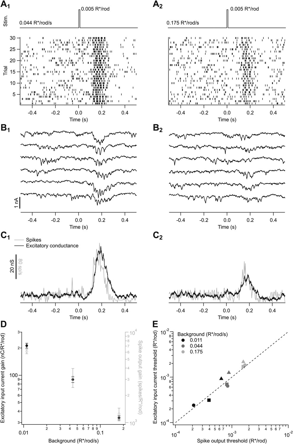
Adaptation is engaged at dim backgrounds in both excitatory inputs and spike outputs from On parasol cells.
(A)–(C) responses from an individual On parasol ganglion cell to dim flashes at two different backgrounds. (A1) Light stimulus (top, 20 ms flashes at 0 s) and raster of the cell’s spike response to several stimulus trials. (B1) Excitatory synaptic currents in response to the same stimulus. (C1) Mean spike rate and excitatory conductance. (A2)–(C2) responses to the same flash as in (A1–C1) but delivered on a higher background. (D) Gain of the excitatory input current and spike output as a function of background for the cell in (A–C). Gain of the excitatory currents was measured by integrating the current over time and dividing by the flash strength, and hence has units of nC/R*/rod/s. Gain of the spike responses was measured by integrating spikes over time. Error bars are SD (n = 20–30 trials). (E) Detection threshold (see ‘Materials and methods’) calculated from excitatory input current and spike output for three different cells (symbols) at three backgrounds each (gray scale). Dashed line represents unity.
Figure 3
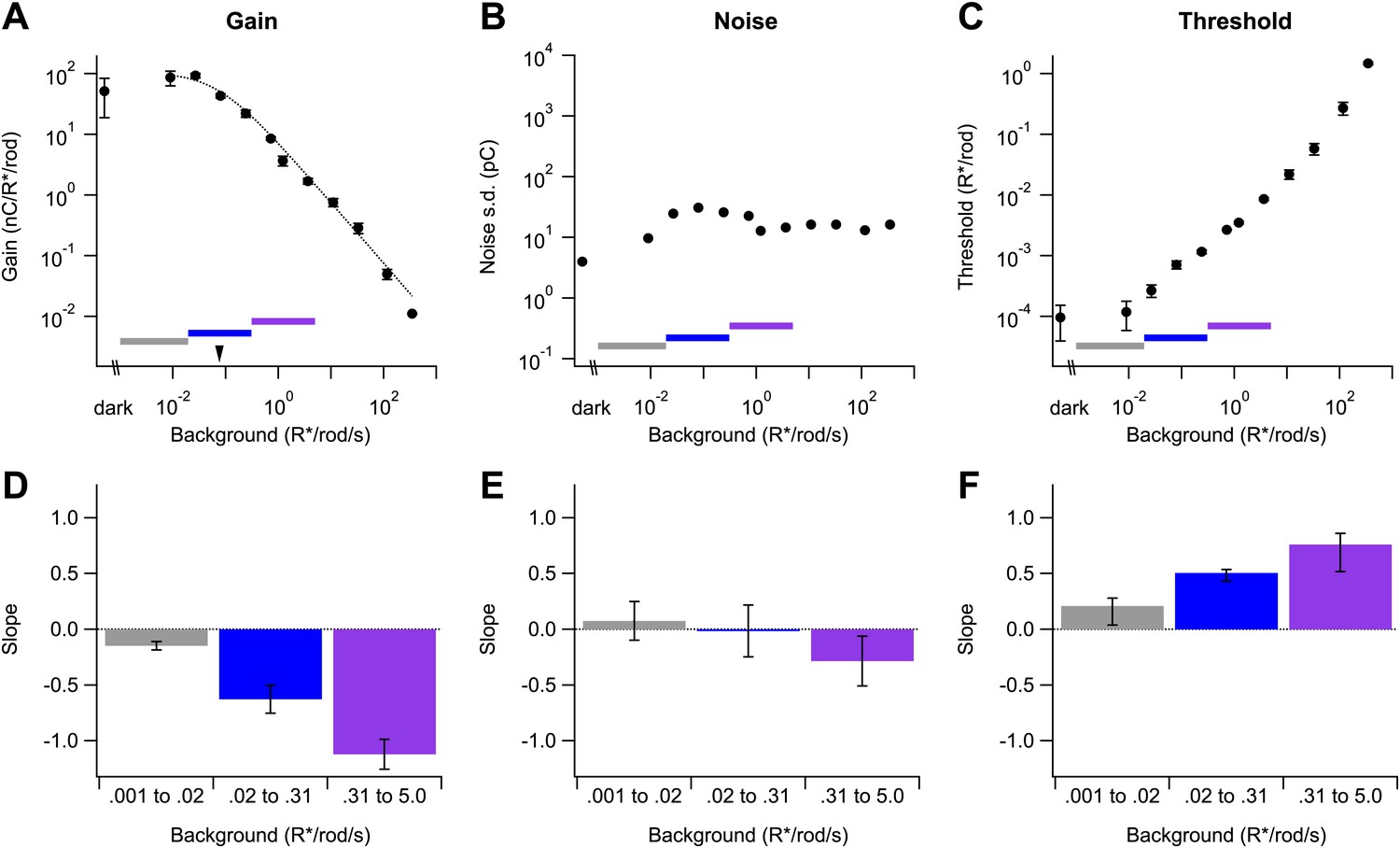
Changes in gain, noise, and threshold with background.
(A)–(C) Example data from a single cell showing gain of the dim flash response (A), noise (B), and threshold (C) as a function of background (see ‘Materials and methods’). Error bars (A and C) are standard deviations across two flash strengths. Colored bars indicate background segments in which the slope was computed. Dotted line (A) represents the fit of a modified Weber function with the half-desensitizing background indicated by an arrowhead (see Equation 1). (D)–(F) Population data reporting the slope of each parameter on a log–log scale in three background regions. Error bars are SD (n = 4, 6, and 5 cells in each background segment).
Figure 4
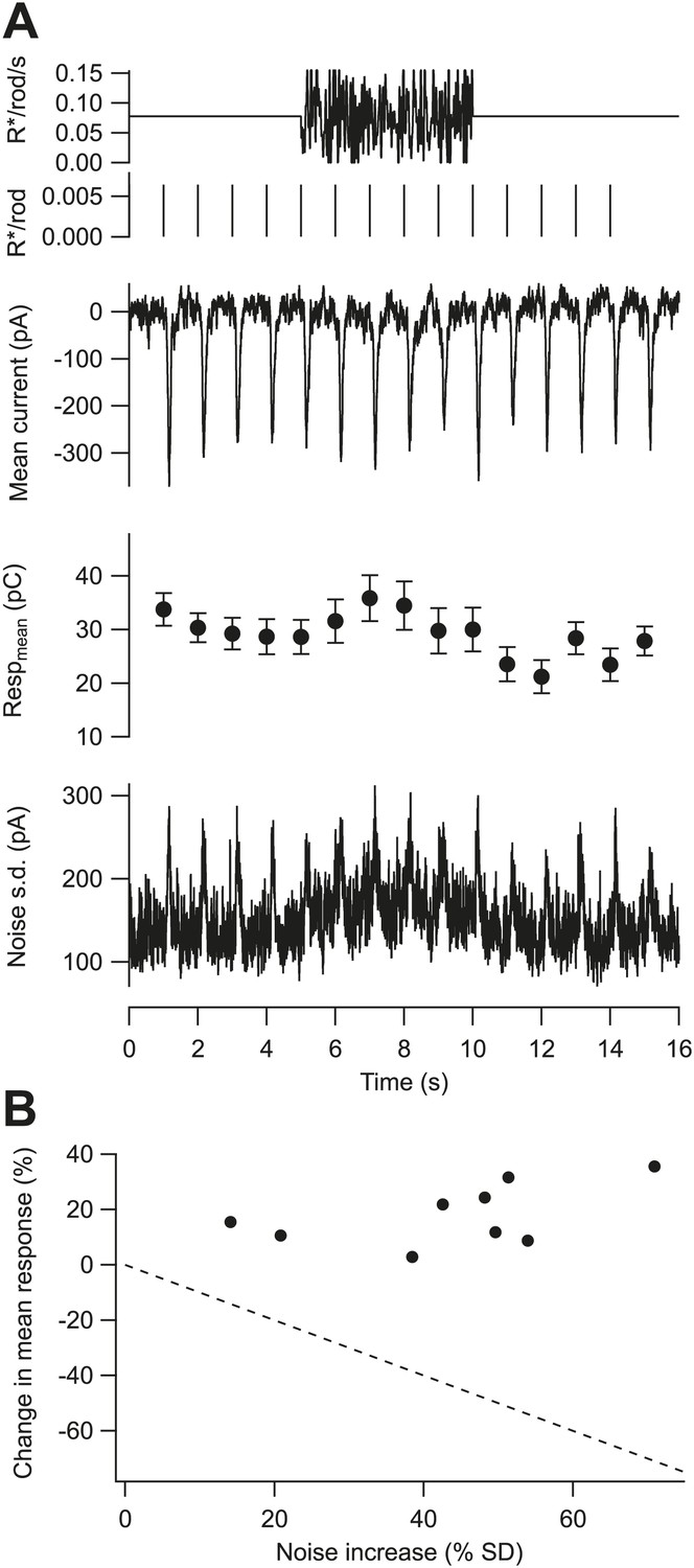
Gain is controlled by the mean not the variance of the background.
(A) Fluctuating background experiment for an example cell. From top: background, probe flashes, mean excitatory input current, mean and SEM of each flash response (n = 10 trials), and standard deviation of the current. (B) Change in the mean of the flash response plotted against the change in the standard deviation of the baseline current caused by the fluctuating background for nine cells. Dashed line indicates the prediction for a gain control mechanism based on the noise of the background—that is, if gain was inversely proportional to the standard deviation.
Figure 5 with 1 supplement
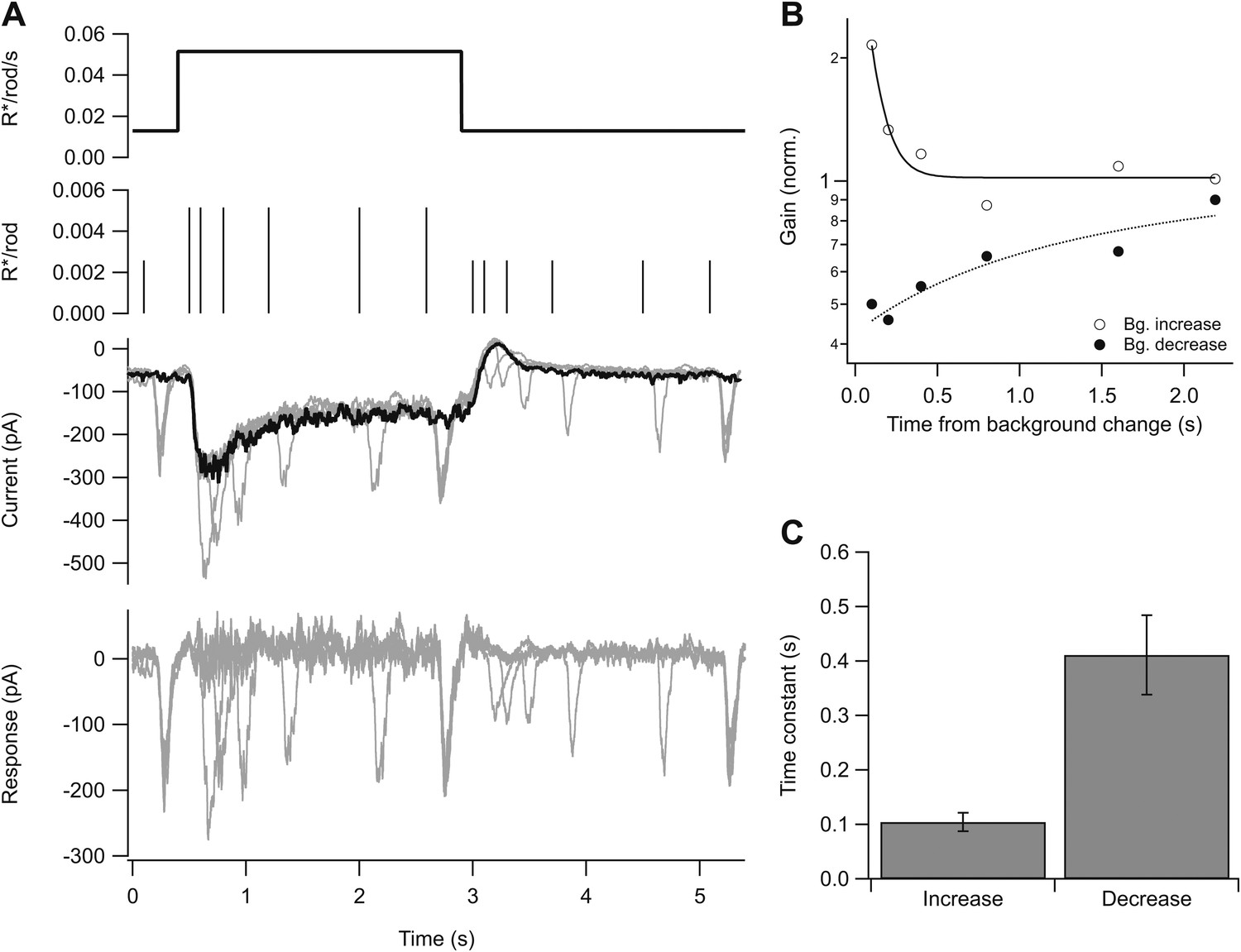
Kinetics of gain control.
(A) From top: background, probe flashes, current traces for each probe flash set (see ‘Materials and methods’) and for the background alone (black), response obtained by subtracting the background step trace from each test response. Five test flashes where given in each epoch: two at variable times following background step onset and offset, and three at fixed times before the step, at the end of the step, and at the end of the epoch. (B) Gain change (on a logarithmic scale) as a function of the time of the probe flash following an increase or decrease in background. Lines are single exponential fits. (C) Time constant of the fit as in (B) across a population of cells. Error bars are SEM (n = 5).
Figure 5—figure supplement 1
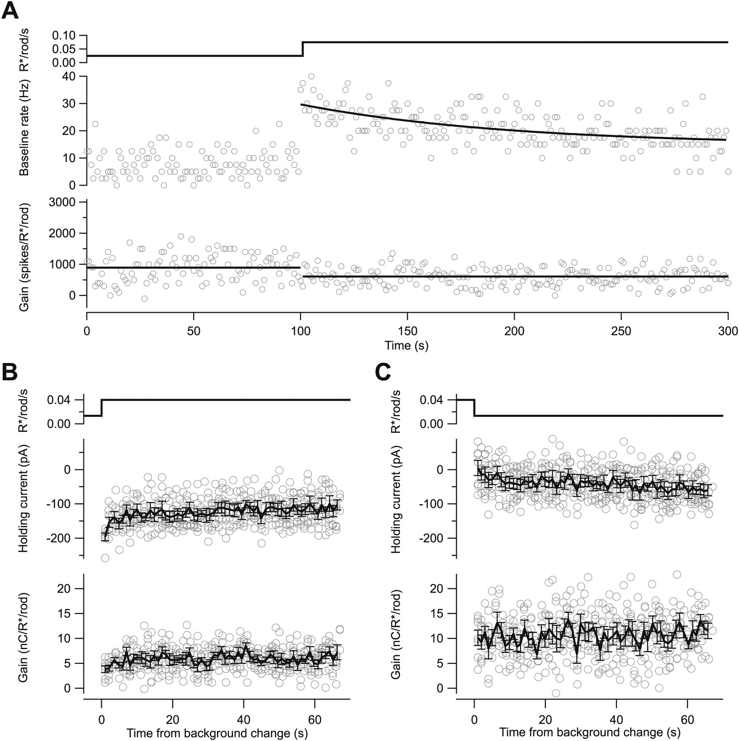
Kinetics of changes in baseline and gain differ.
(A) Baseline spike rate (middle) and gain of response to a brief flash (bottom; as in Figure 2). Black line (middle) is an exponential fit with a time constant of 97 s; lines (bottom) are mean gain value at each background. (B) and (C) Changes in the holding current (middle) and gain (bottom) following an increase (B) or decrease (C) in background from whole-cell recordings with a holding potential of −70 mV. Changes in holding current reflect changes in the tonic excitatory synaptic input to the cell. Gain changed within a few seconds of a change in background (i.e., the ∼twofold change in gain between the left and right panels is already present in the first few flash responses). Black lines are mean ± SEM across seven repeats of the background step.
Figure 6
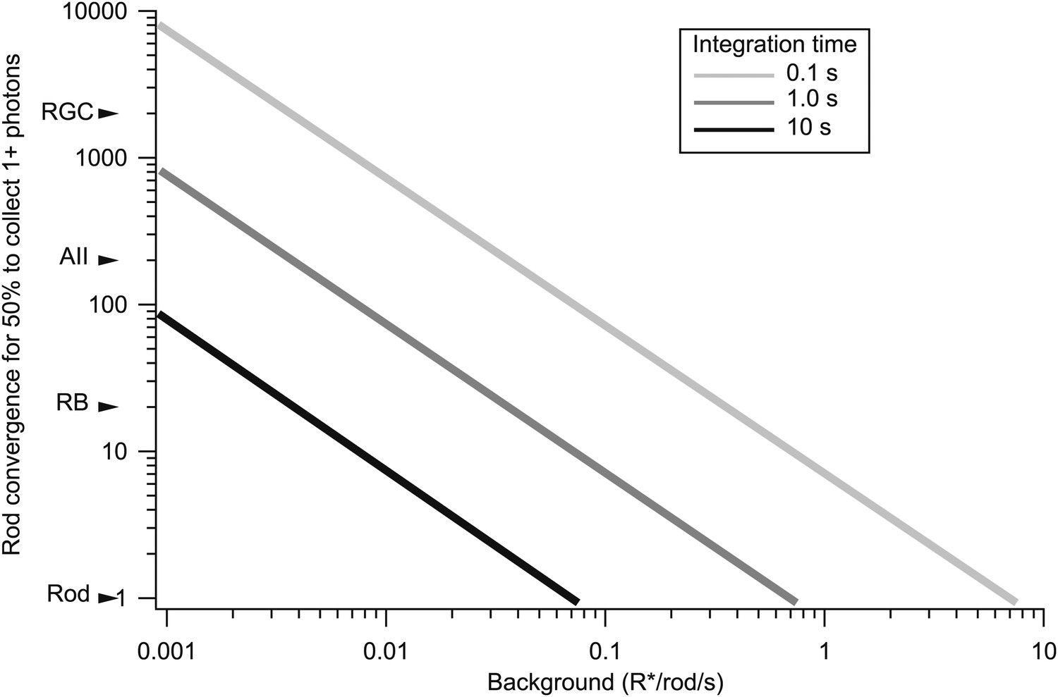
The trade-off between rod convergence and integration time in gain control.
Rod convergence required for 50% of the neural elements to collect one or more photons is plotted as a function of background (see ‘Materials and methods’). Estimated convergence along the rod bipolar pathway is indicated along the y-axis. AII: AII amacrine cell; CB: On cone bipolar cell; RB: rod bipolar cell; RGC: peripheral parasol retinal ganglion cell.
Figure 7
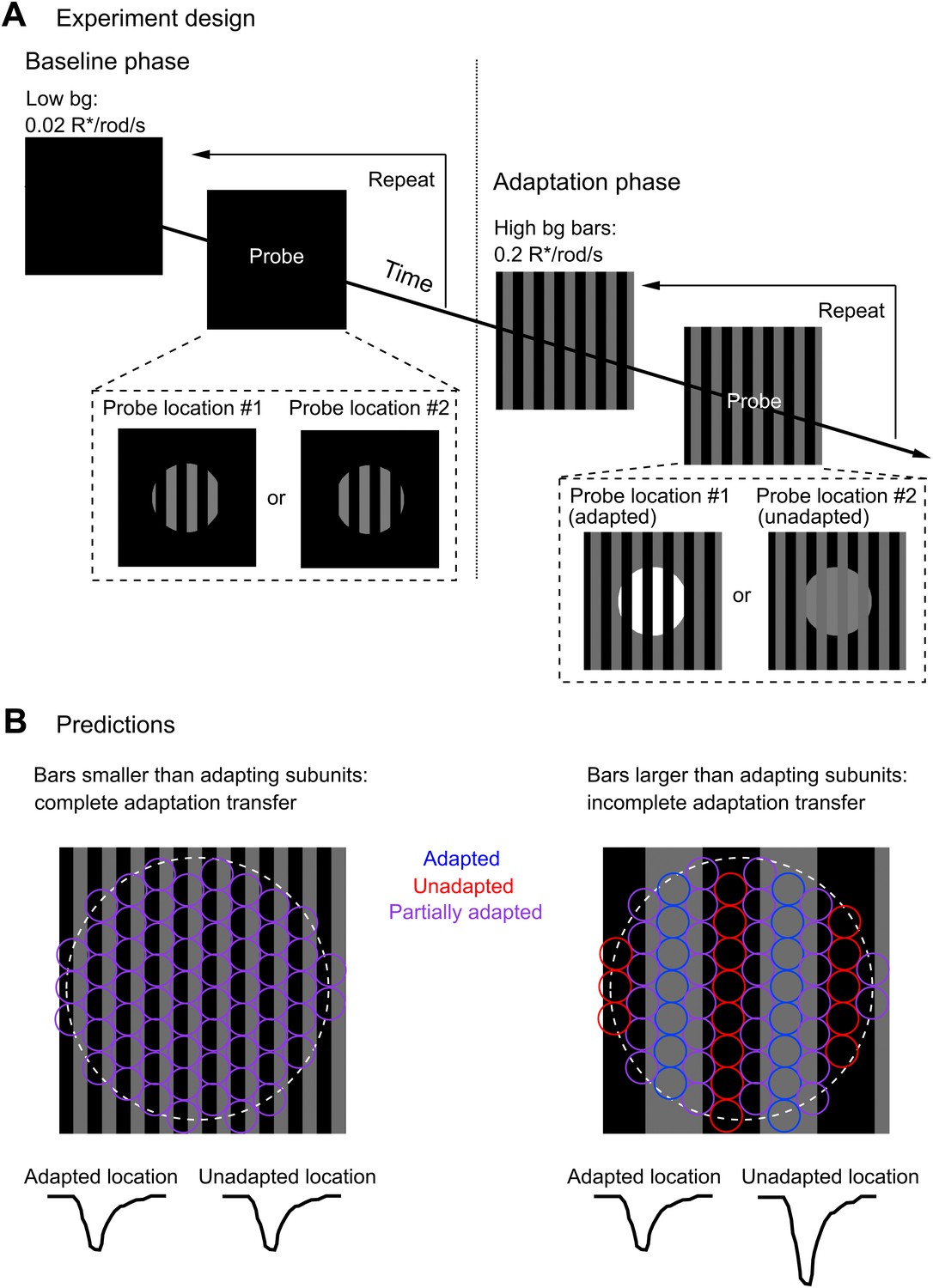
Measuring the spatial scale of gain control.
(A) Diagram of the experimental design. The baseline phase consisted of at least 20 trials each of two probe patterns flashed on a uniform dim background (0.02 R*/rod/s). In the adaptation phase, the same two probe patterns were presented superimposed on an adapting background of bars of higher intensity (0.2 R*/rod/s), again for at least 20 trials each. One probe location was aligned with the adapting bars (adapted location), whereas the other was out of phase (unadapted location). (B) Repeating the experiment with a variety of adapting bar sizes tests the spatial scale of adaptation. Bars up to half the diameter of the adapting subregion of the receptive field would be expected to cause a complete transfer of adaptation from the adapted to the unadapted location. Bars wider than the diameter of the adapting subregion would be expected to cause incomplete adaptation transfer.
Figure 8
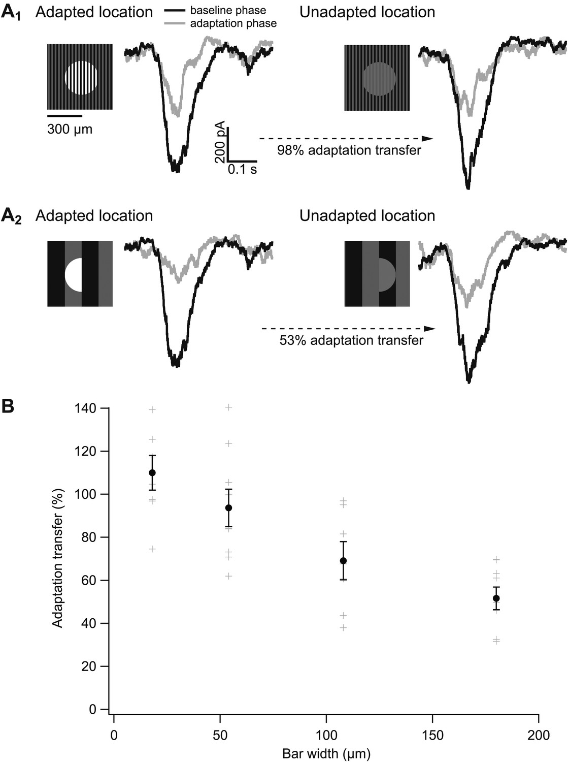
The spatial scale of gain control.
(A) Responses of an example cell to probes during the baseline phase (black) and the adapting phase (gray) of the experiment at both the adapted and unadapted locations. Adapting bars were 18 μm wide in (A1) and 180 μm wide in (A2). (B) Adaptation transfer as a function of the width of the adapting stripes. Gray symbols are individual cells and black points are mean and SEM (n = 7, 9, 7, and 8 for bar widths in ascending order).
Figure 9
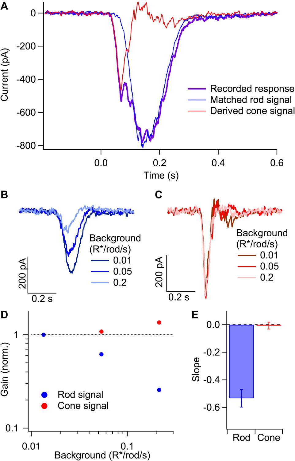
Gain control in rod and cone pathways.
(A) Response to long-wavelength light (purple) and matched response to short-wavelength light (blue) were used to derive the isolated cone response (red). (B) Rod responses to the same flash intensity at three different backgrounds. (C) Cone responses recorded in the same cell as in (B). (D) Gain of the rod and cone responses for the cell in (B and C) plotted against the background on a log–log scale. Gain values have been normalized by the gain at the lowest background. (E) Slope of the background vs gain function on a log–log scale for rod and cone responses in the same population of cells. Error bars are SEM (n = 7).
Figure 10

Gain control is stable and reproducible in spike responses. Spike responses from an example On parasol cell in primate retina.
(A) Background light level. (B) Increase in spike count following a 10-ms flash (i.e., with the maintained spike rate before the flash subtracted). The test flash strength is indicated by the gray line and the right axis. Flashes were presented at 1-s intervals beginning 1 s after each background change. (C) Gain of the spike response in spikes per isomerization per rod (R*/rod). Gain was calculated by dividing the spike count in (B) by the flash strength. (D) Baseline spike rate measured prior to each flash.
Figure 11
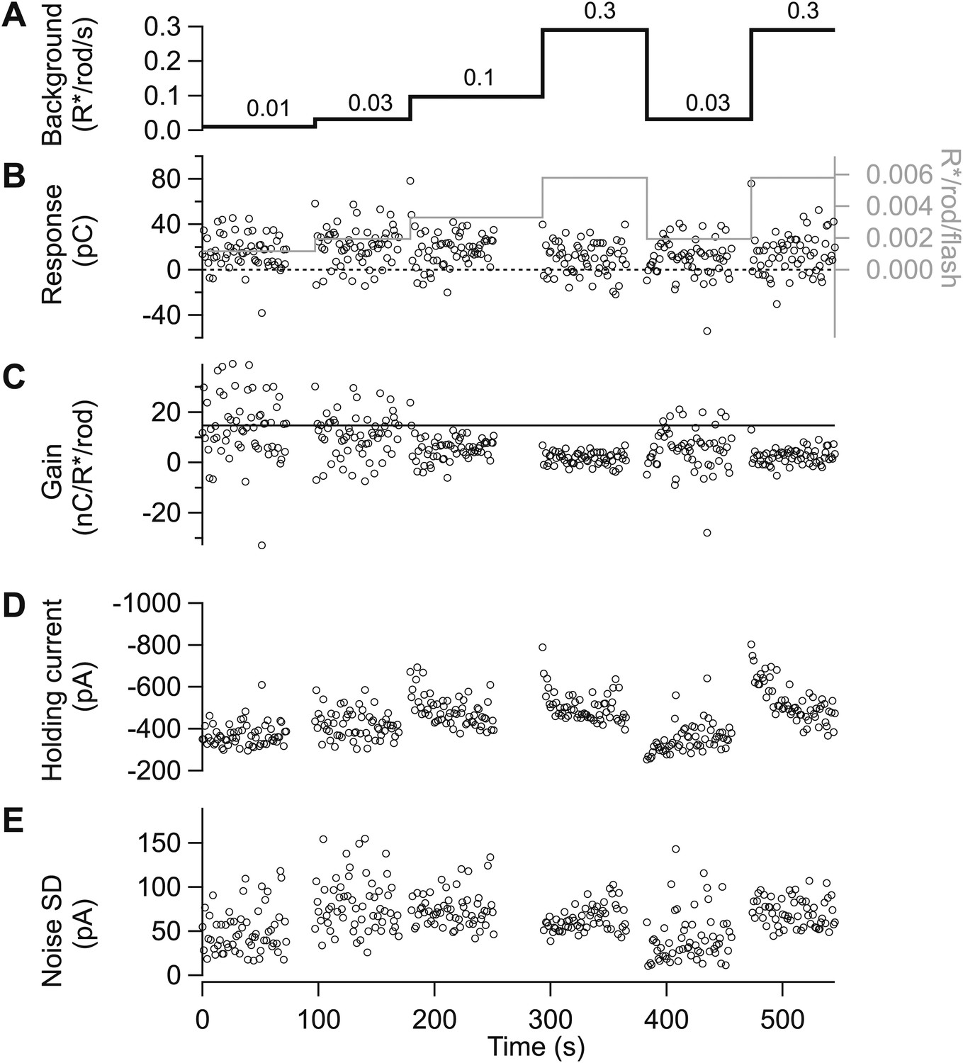
Gain control is stable and reproducible in excitatory input currents.
(A)–(D) Excitatory synaptic currents following the same format as Figure 10. Data are from a different cell voltage clamped at −70 mV, the approximate reversal potential for inhibitory input. (E) Standard deviation of the current in the time interval preceding each flash.
Download links
A two-part list of links to download the article, or parts of the article, in various formats.
Downloads (link to download the article as PDF)
Open citations (links to open the citations from this article in various online reference manager services)
Cite this article (links to download the citations from this article in formats compatible with various reference manager tools)
Controlling gain one photon at a time
eLife 2:e00467.
https://doi.org/10.7554/eLife.00467


