Viral genome structures are optimal for capsid assembly
- Brandeis University, United States
Figures
Figure 1
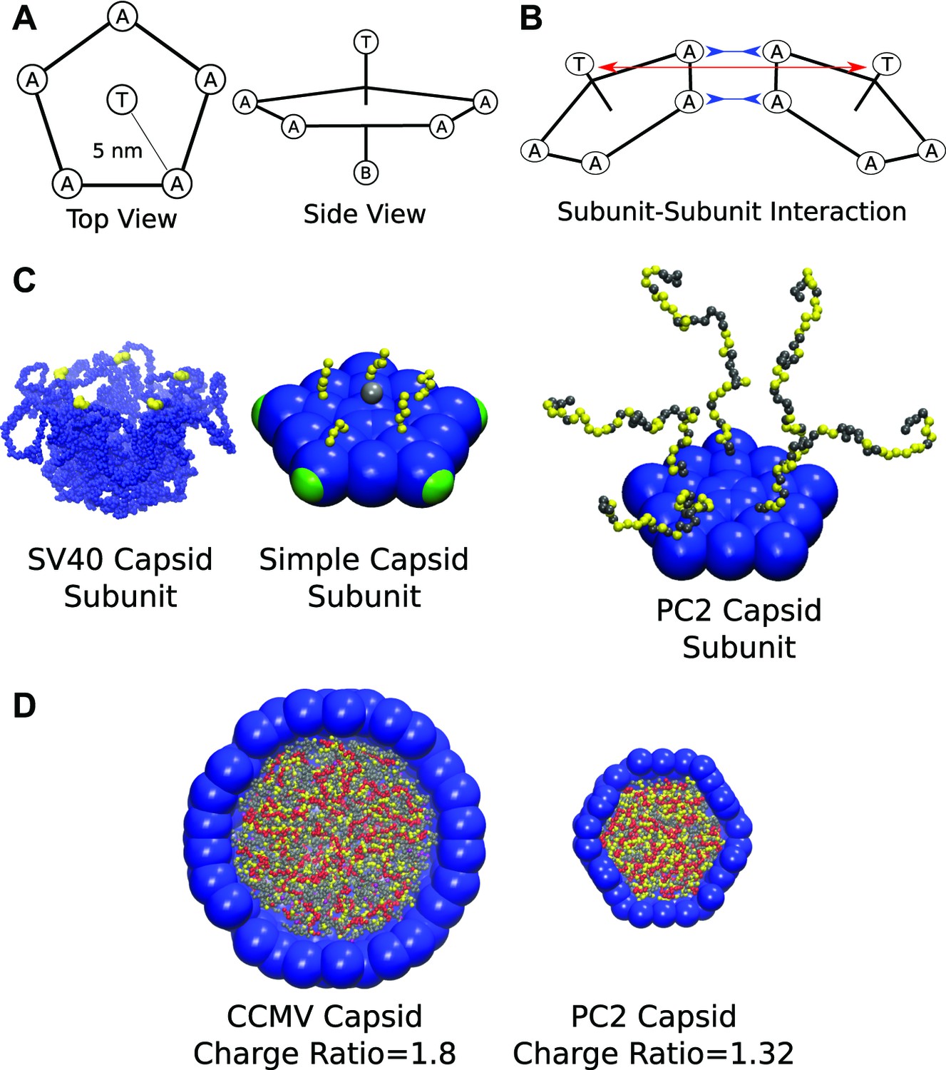
Schematics and representative images of model systems. (A), (B) Model schematic for (A) a single subunit, and (B) two interacting subunits, showing positions of the attractor (‘A’), Top (‘T’), and Bottom (‘B’) pseudoatoms, which are defined in the ‘Model’ section and in the ‘Methods’. (C) (left) The pentameric SV40 capsid protein subunit, which motivates our model. The globular portions of proteins are shown in blue and the beginning of the NA binding motifs (ARMs) in yellow, though much of the ARMs are not resolved in the crystal structure (Stehle et al., 1996). Space-filling model of the basic subunit model (middle) and a pentamer from the PC2 model (right). (D) A cutaway view of complete CCMV and PC2 capsids (with respective biological charge ratios of 1.8 and 1.32). Beads are colored as follows: blue = excluders, green = attractors, yellow = positive ARM bead, gray = neutral ARM bead, red = polyelectrolyte.
Figure 2 with 2 supplements
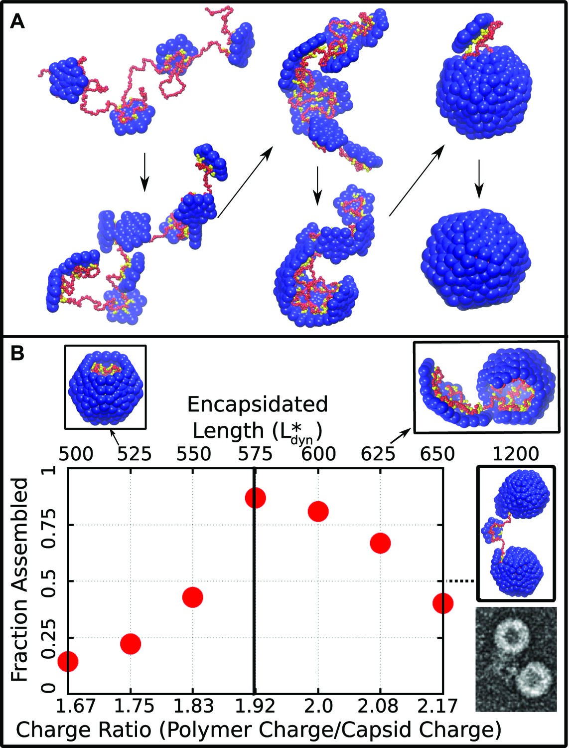
Capsid assembly around a linear polyelectrolyte. (A) Snapshots illustrating assembly of subunits with ARM length = 5 around a linear polyelectrolyte with 600 segments. Beads are colored as in Figure 1. (B) Fraction of trajectories leading to a complete capsid as a function of polymer length (top axis) or charge ratio (bottom axis). The dashed line indicates the thermodynamic optimum charge ratio or length from equilibrium calculations. Snapshots of typical outcomes above and below the optimal length are shown. (Far right) A typical assembly outcome for polymer length 1200 (twice ) is compared to an EM image of CCMV proteins assembled around an RNA which is twice the CCMV genome length (image extracted from panel C of Figure 5 in Cadena-Nava et al., 2012).
Figure 2—figure supplement 1

Estimation of the critical nucleus size.
As in Kivenson and Hagan (2010), we define the critical nucleus size as the smallest cluster of subunits for which more than 50% of trajectories proceed to complete assembly before complete disassembly (defined as reaching a state of ). This plot, which is for trajectories with a linear polymer of length 575, indicates .
Figure 2—figure supplement 2
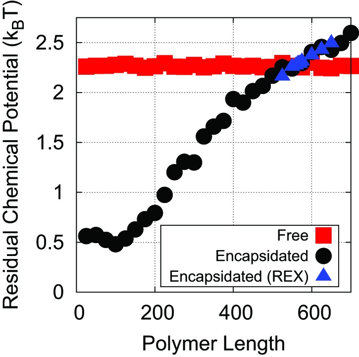
The residual chemical potential calculated by the Widom test-particle insertion method.
Here, the residual chemical potential is shown for a linear polyelectrolyte, isolated in solution (red squares) and encapsidated in the simple capsid model (Figure 1) (black circles). Results from replica exchange (REX) simulations on the encapsidated polymer are also shown (blue triangles).
Figure 3 with 3 supplements
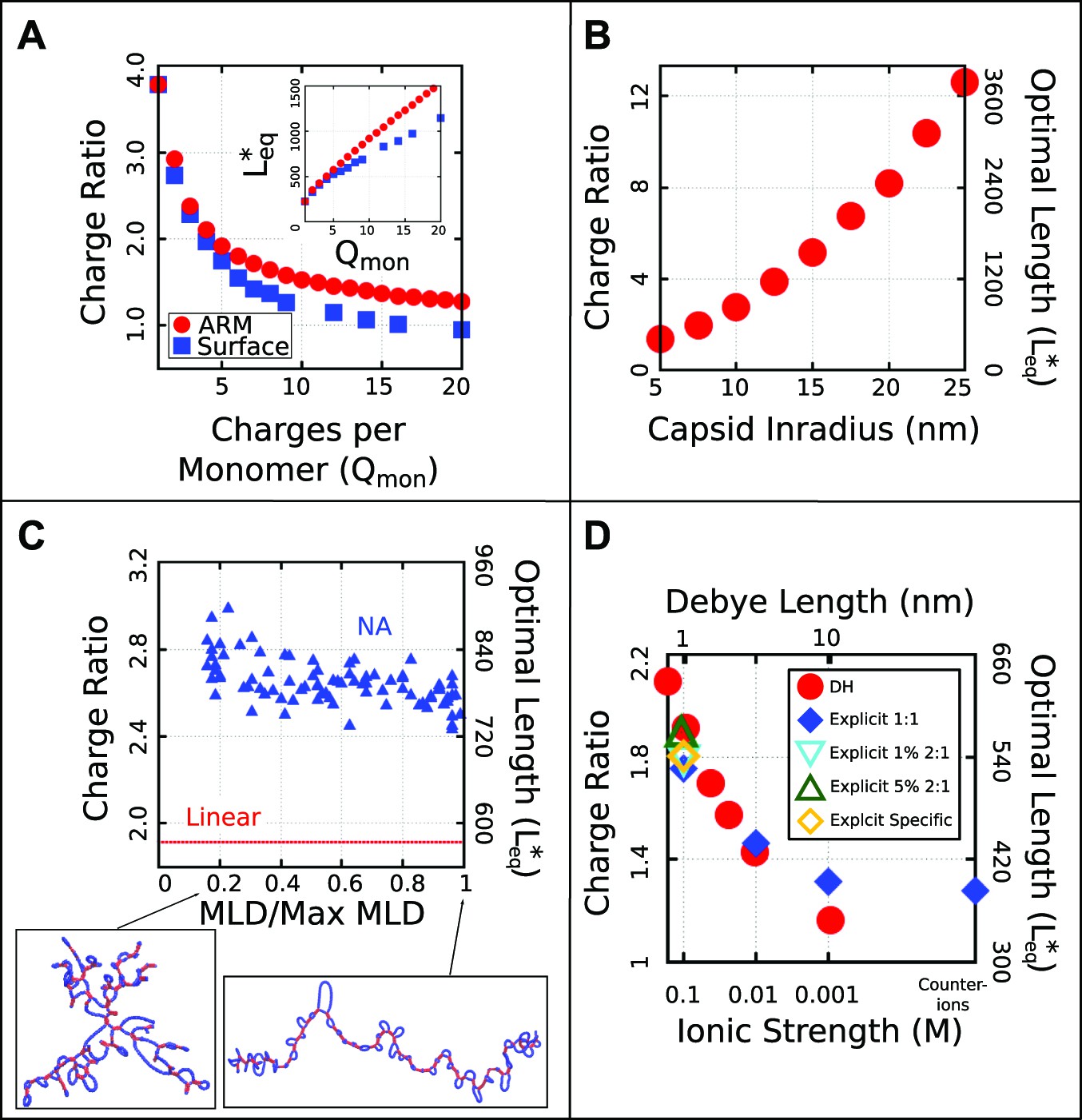
Effect of control parameters on the thermodynamic optimal length and charge ratio.
(A) Effect of increasing capsid charge, with capsid nm. (B) Effect of increasing capsid size for fixed ARM length = 5. (C) Effect of base-pairing, with base-paired nucleotides and varying maximum ladder distance (MLD), for capsid nm and ARM Length = 5. Snapshots of our model NA structures with small and large MLD’s are shown (prior to encapsidation), with double-stranded regions in red and single-stranded regions in blue. The result for no base-pairing (linear) is shown as a dashed line. (D) Effect of ionic strength and comparison between Debye–Huckel interactions and explicit ions. The thermodynamic optimum lengths and corresponding optimal charge ratios are shown as functions of the ionic strength (Debye screening length), calculated with simulations using Debye–Huckel (DH) interactions (red circles) or Coulomb interactions with explicit ions, 1:1 salt and no divalent cations (blue diamonds), 1% 2:1 salt (blue triangles), or 5% 2:1 salt (green triangles). An additional system with monovalent free ions and divalent cations irreversibly bound to the polyelectrolyte is also presented (yellow diamonds, see ‘Model potentials and parameters’). Calculations were performed using the simple capsid model (Figure 1) and a linear polyelectrolyte.
Figure 3—figure supplement 1

The thermodynamic optimum lengths and charge ratios monotonically decrease with increasing persistence length for a linear, semiflexible polyelectrolyte.
While this observation could be anticipated on intuitive grounds, the quantitative decrease is substantial—a 32 % decrease in optimal charge ratio between our most flexible polymer ( nm) and our stiffest polymer ( nm). The persistence length is obtained by simulating the polymer unencapsidated in solution and fitting the segmental autocorrelation function to an exponential decay, where the persistence length is the decay constant. The simulations were performed using the simple capsid model (Figure 1, with dodecahedron inradius , and an ARM length of 5 positive charges). Representative snapshots of the encapsidated polymer (taken from simulations at the optimal length) are shown for several persistence lengths. The capsid and ARMs are rendered invisible in these snapshots to enable visibility of the polyelectrolyte.
Figure 3—figure supplement 2
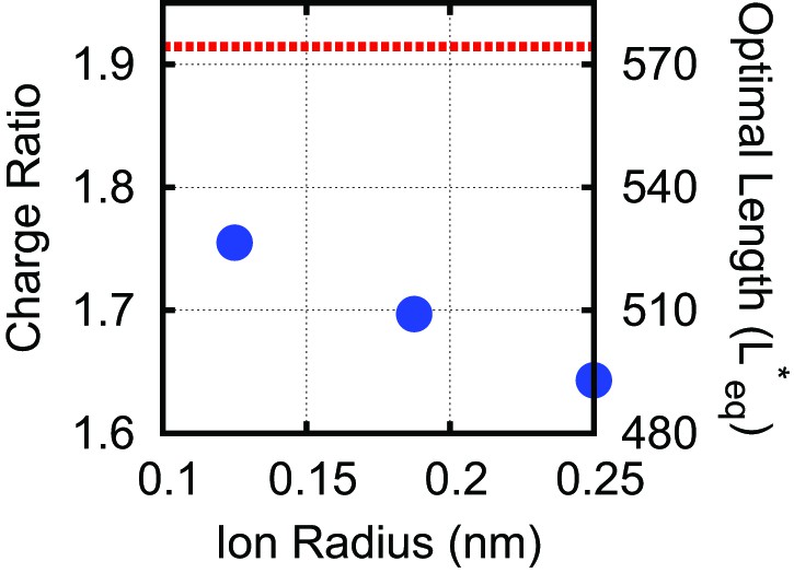
Effect of varying the ion radius.
Explicit ions (blue circles) are varied in size at 100 mM monovalent ions, compared with the DH result (dashed red line).
The explicit ion results approach those of the Debye–Huckel model simulations at physiological salt concentrations (100 mM) as the explicit ion radius is decreased, since ion excluded-volume is reduced, with the two methods agreeing to within 10% for the most realistic ion radius (0.125 nm). Note, in Figure 3D all ion radii were set to 0.125 nm.
Figure 3—figure supplement 3
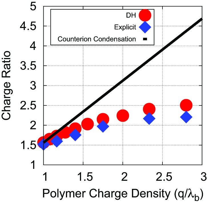
Effects of counterion condensation on .
In a previous work (Belyi and Muthukumar, 2006) it was noted that the high charge densities of RNA and peptide tails will give rise to counterion condensation, where the linear charge density of a polyelectrolyte is renormalized by condensed counterions to an effective linear charge density of charges/nm, with nm as the Bjerrum length. We chose not to charge renormalize in our simulations which used the Debye–Huckel model because association of RNA or an anionic linear polyelectrolyte with the oppositely charged peptide tails will lead to dissociation of condensed counterions. To test the validity of this choice (and to further test the validity of the Debye–Huckel model), we calculated optimal lengths as a function of the linear charge density for a linear polyelectrolyte using both the Debye–Huckel (with no assumed counterion condensation red circles) and Coulomb interactions with explicit counterions (blue diamonds). In the latter simulations counterion condensation arises naturally and responds to local charge densities with no approximations. The linear charge density was varied by adjusting the equilibrium bond lengths between neighboring beads in the polyelectrolyte; all other parameters were unchanged. The results are compared to the results of simulations with the Debye–Huckel model and irreversible counterion condensation (black line). To obtain this result, we performed a single simulation using the Debye–Huckel model with a linear charge density of 1 , and then assumed all charge densities exceeding this value are renormalized, so that the optimal charge ratio increases proportionally with the bare linear charge density. That is, at a charge density of 2 , only half the polymer is effectively charged and the optimal charge ratio (calculated as a ratio of bare charge on the RNA to bare charge on the peptide arms) doubles. The simulations used the simple capsid model (, ARM Length = 5) at a Deybe length of nm or a salt concentration of 100 mM, respectively.
Figure 4 with 2 supplements
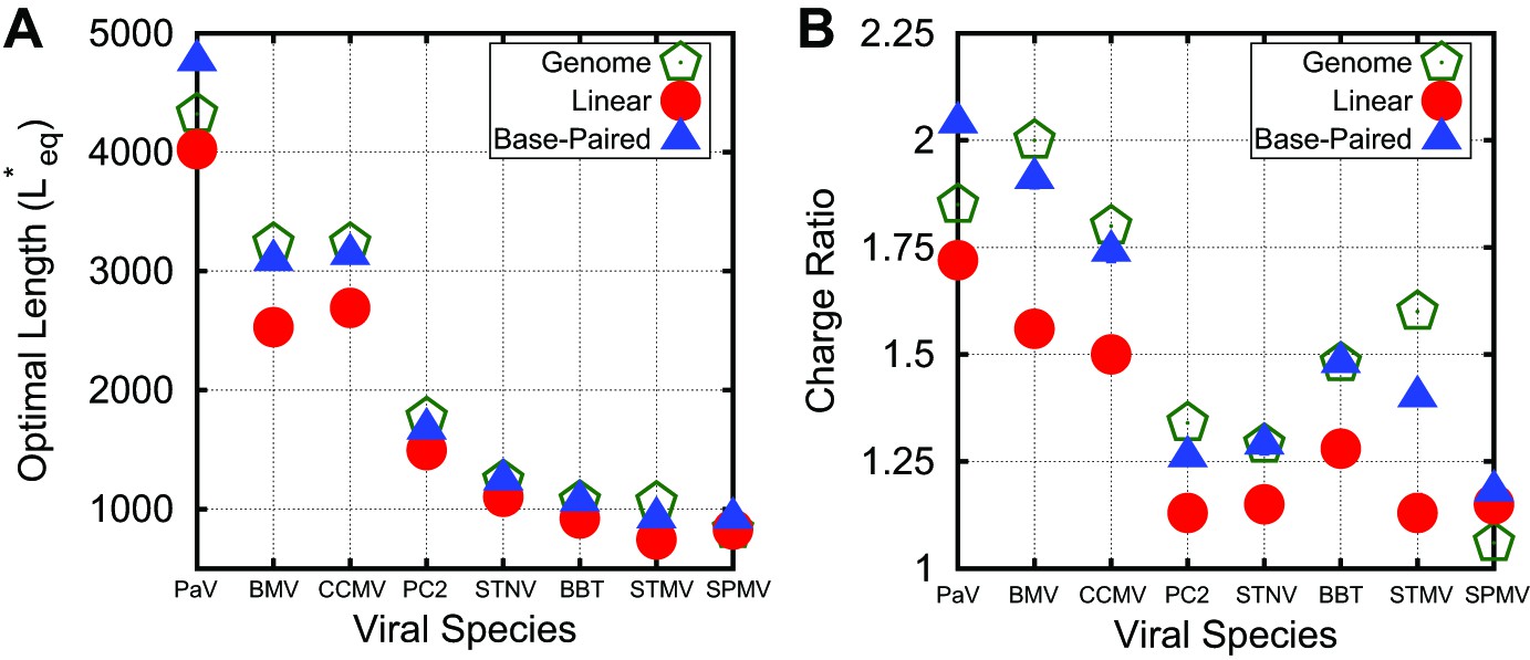
Correspondance between viral genomes and model calculations. Comparison between viral genome lengths and calculated thermodynamic optimal lengths (A) and charge ratios (B) for models based on the indicated viral capsid structures (see Table 1). Predicted optimal lengths are shown for linear polyelectrolytes (red circles) and model NAs (blue triangles) with 50% base-pairing. Viral genome lengths are shown with green pentagons symbols. Error bars fall within the symbol sizes.
Figure 4—figure supplement 1
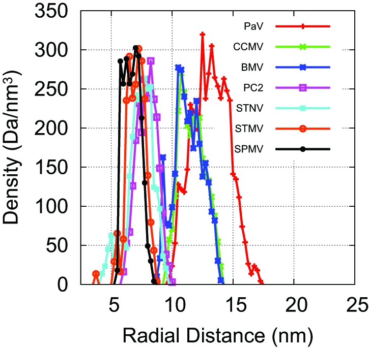
Our capsid model can be modified to describe specific viral capsids by altering the capsid radius and ARM sequence.
Atomic-resolution structures of capsids are available for PC2, STNV, STMV, SPMV, PaV, BMV, and CCMV (Jones and Liljas, 1984; Ban and McPherson, 1995; Speir et al., 1995; Larson et al., 1998; Tang et al., 2001; Lucas et al., 2002; Khayat et al., 2011). For each capsid structure, we estimated the radius by fitting the radial density of capsid protein (C, N, S, O atoms), as plotted here, to a Gaussian. For capsids, we scaled the inradius of our dodecahedral model capsid (Figure 1) until its interior volume was equal to the volume of a sphere with the radius of the biological capsid. The ARMs were anchored as shown in Figure 1, midway across the pentagonal radius (we found that changing the locations of anchor points did not substantially affect ), and the sequence of positive, negative, and neutral beads was set to match the amino acid sequence of the capsid protein for the virus being modeled. For capsids, an icosahedrally symmetric capsid was designed with the excluders and ARMs placed based on the crystal structure of the Brome Mosaic Virus (Lucas et al., 2002). For other viruses the ARM sequence and capsid radius were adjusted. For the satellite viruses, there are basic residues located on the capsid inner surface (in addition to those found in the ARM); for each such residue a positive charge was rigidly fixed to the inner surface of the model capsid. No atomic-resolution structures for capsids of viruses in the Nanoviridae family are available, so the capsid radius for BBT was based on electron microscopy (Harding et al., 1991).
Figure 4—figure supplement 2
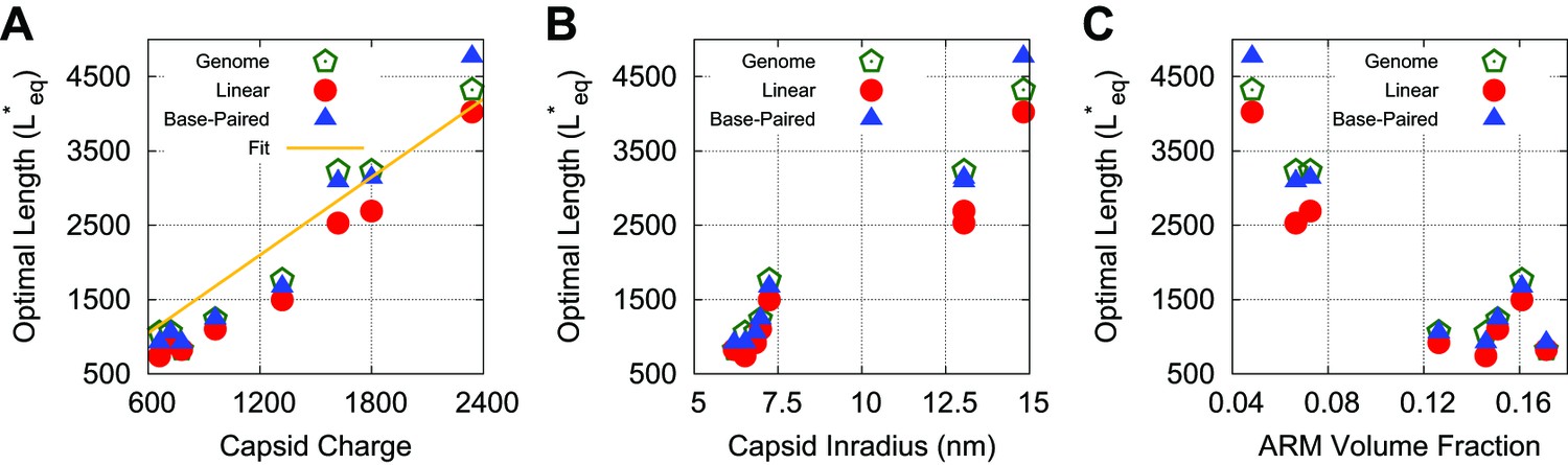
Optimal lengths are sensitive to multiple factors.
Values of the thermodynamic optimum length for the capsids considered in Figure 4 plotted against (A) total capsid charge, (B) capsid inradius, (C) ARM volume fraction. Values are shown for a linear polyelectrolyte, the model base-paired NA, and the actual genome length for each virus. In panel (A) we find that a linear fit yields a slope similar to that previously observed (1.75), which we present as a comparison (Belyi and Muthukumar, 2006).
Figure 5 with 4 supplements
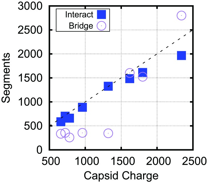
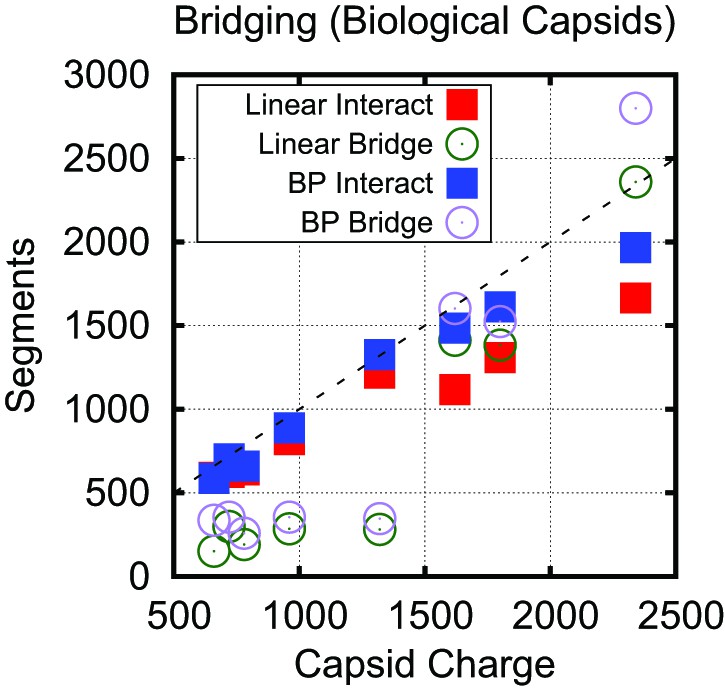
Bridging in biological capsids. Number of NA segments that directly interact with positively charged ARM segments (interaction energy , blue squares) and bridging segments (interaction energy , purple circles).
The numbers are calculated at the optimal length for each capsid shown in Figure 4 using the base-paired model. For visual reference, the dashed line indicates a 1:1 correspondence between capsid charge and number of nucleotides.
Figure 5—figure supplement 1
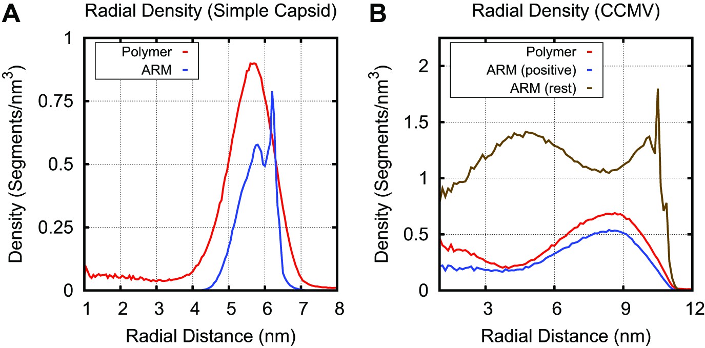
Radial density for linear polymer and ARM segments in the simple capsid (A) and CCMV (B).
The sharp peak in ARM density is due to the first ARM segment, which is rigidly attached to the capsid shell. In the simple capsid the polymer segments are concentrated within a few nm of the capsid shell, with lower densities in the capsid center. For CCMV, the longer arms result in a more diffuse distribution of positive charges within the capsid interior as compared to the basic capsid model. While there is some co-localization of positively charged ARM and combined neutral and negatively charged polymer segments, their densities peak at slightly different radii. The CCMV ARM sequence contains 48 segments, with 11 positive segments and 1 negative segment. Though the charges are not homogenously distributed throughout the sequence (9 occur within a 19 segment stretch), the degree of separation observed was unexpected.
Figure 5—figure supplement 2
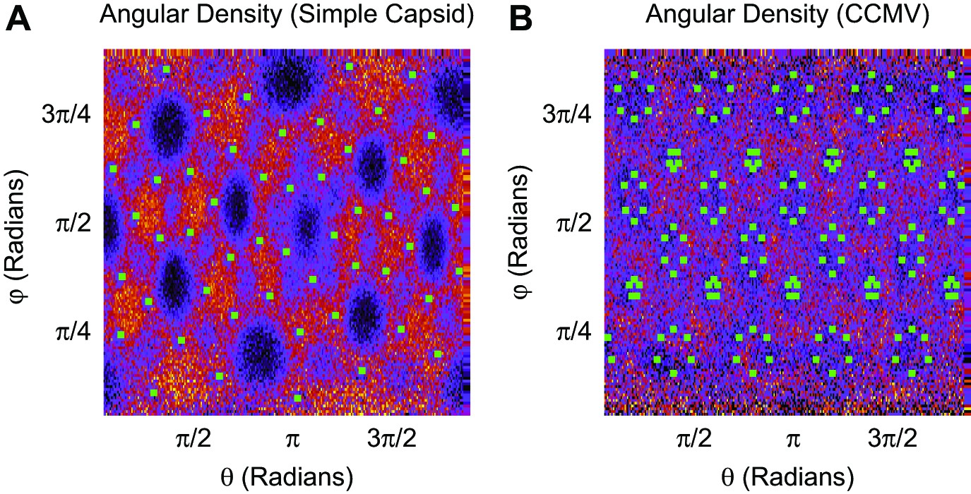
Angular density of linear polymer segments (heat map) in the basic capsid model (A) and CCMV (B).
Green squares indicate the first ARM segment. Segment densities are averaged over radial distances of 5–6.25 nm (A) and 8.75–10 nm (B), as a function of the spherical angles, without angular averaging. For the simple capsid, the polymer more frequently resides in the vertices between subunits (between the clusters of 3 ARMs) as well as along the dodecahedral edges, and resides less frequently in the center of the subunit faces. The angular density is heterogeneous in CCMV, though to a lesser extent than found for the simple capsid.
Figure 5—figure supplement 3
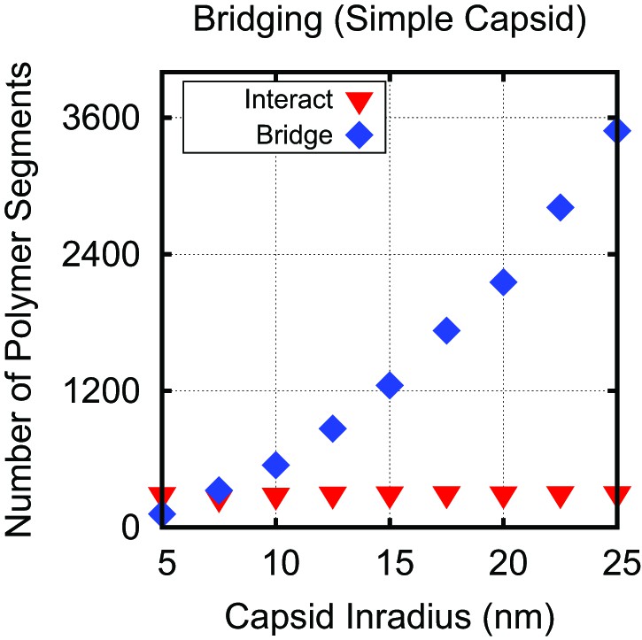
Capsid radius and polymer bridging.
Number of polymer segments interacting with positive capsid charges (red inverted triangles), and number of polymer segments not interacting with positive charges (bridging segments, blue diamonds), using threshold interaction distance of 0.74 nm, which corresponds to a screened electrostatic interaction of . The numbers are calculated at the optimal polymer length as a function of capsid inradius for the simple capsid with constant ARM length (Figure 3B). The number of polymer segments strongly interacting with ARM charges is constant for nm, while the number of bridging segments increases to span the distances between arms. Hence, for capsids with nm, the observed dependence of on capsid size arises entirely due to bridging segments. For smaller capsids, there is a weak increase in the number of interacting segments with size as more conformational space around the ARMs becomes available.
Figure 5—figure supplement 4
Number of NA segments that directly interact with positively charged ARM segments and bridging segments, for both the linear and base-paired model.
For visual reference, the dashed line indicates a 1:1 correspondence between capsid charge and number of nucleotides. This data shows that while the base-paired polymer increases the charge ratio it does so by increasing both the number of segments which are tightly bound and bridging.
Figure 6
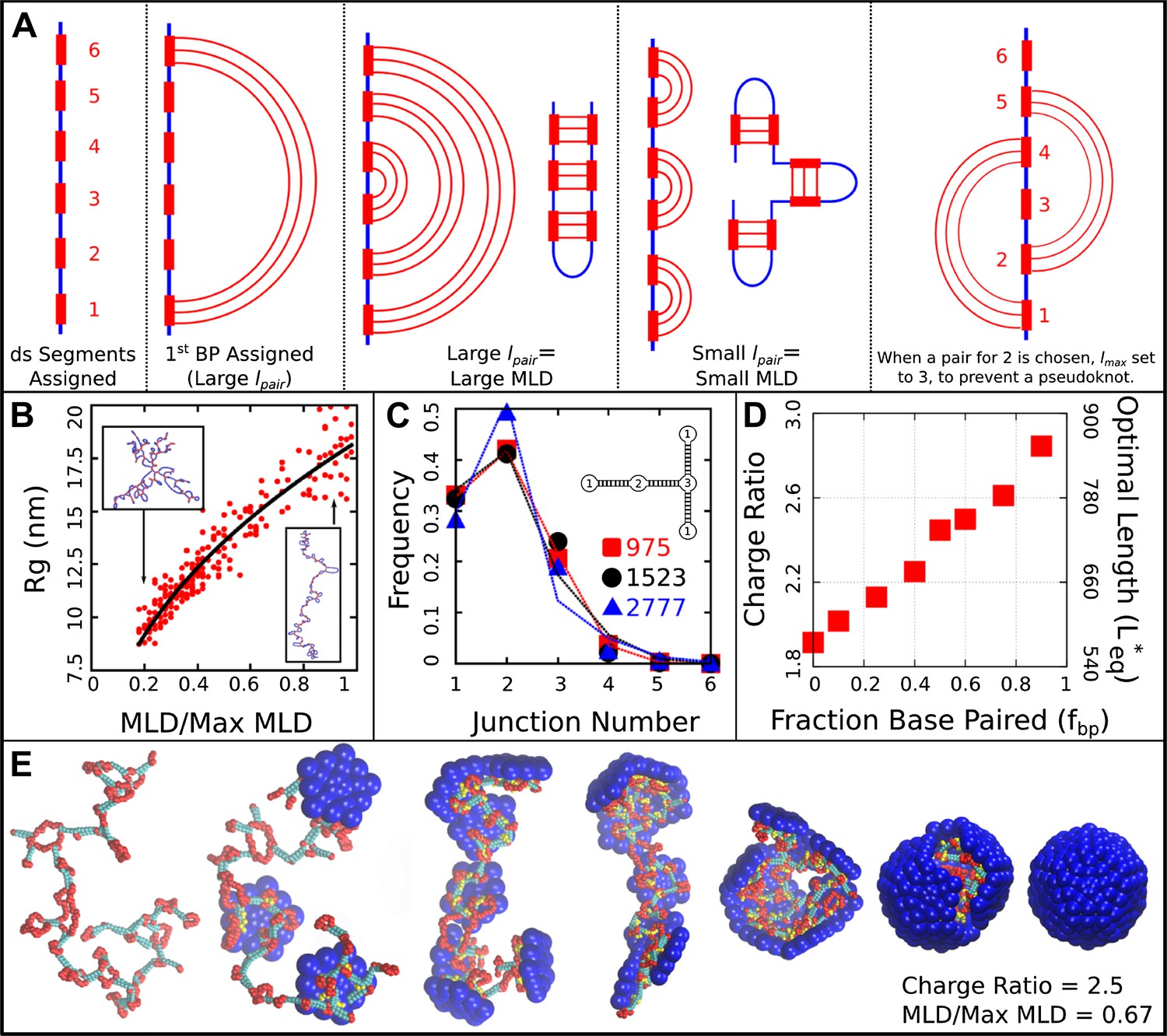
Base-paired polymer setup and analysis. (A) Schematic illustrations of the algorithm we used to obtain a wide range of base-paired structures. From left to right, double-stranded (ds) segments are first randomly assigned. These segments are then base-paired together, starting from one end. If base-paired segments are widely separated (i.e., is large) then subsequent nested base-pairs lead to an extended structure. Conversely, if is small, less extended structures form. The right-most panel indicates a psuedoknot, a structural motif we have prevented from occurring in this model, by setting to the last unpaired segment. (B) Radius of gyration for model NAs isolated in solution as a function of maximum ladder distance (MLD) normalized by the maximum possible MLD. The nucleic acid has 1000 nt, 50% of which are base-paired. (C) The frequency of junction numbers can be altered by varying λ in Equation 2, with large values of λ leading to large values of . The symbols indicate the relative frequency of junction numbers for biological RNAs with indicated lengths, obtained from Ref. (Gopal et al., 2012), and the lines are best fits to these distributions generated by varying λ. The inset illustrates several different junction orders. (D) The thermodynamic optimum length measured for the simple model capsid as a function of the fraction of base-paired nucleotides for a simplified ‘hairpins only’ model (red squares). (E) Snapshots illustrating assembly around a NA. Beads are colored as follows: blue = excluders, yellow = ARM bead, red = single-stranded NA, cyan = double-stranded NA. ‘Top’, ‘Bottom’, and ‘Attractor’ beads removed for clarity.
Videos
Video 1
Capsid Assembly.
Movie illustrating assembly of subunits with ARM length=5 around a linear polyelectrolyte with 600 segments. Beads are colored as in Figure 1.
Video 2
Base-Paired Capsid Assembly.
Movie illustrating assembly of subunits with ARM length=5 around a base-paired molecule with a charge ratio of 2.5 and normalized MLD of 0.67. Beads are colored as in Figure 6.
Tables
Table 1
Details for the models of biological capsids studied in this article. The capsid inradius (distance from capsid center to face center), number of residues in the arginine rich motif (ARM), and net charge of the ARM and inner surface are features used to build these models. The viral genome length is then presented for comparison to the value of predicted for the base-paired model. Finally, the fraction of occupied volume within the capsid is given for the base-paired model at the optimal length
| Virus | Inradius (nm) | ARM Length/Net charge | Genome length | Occupied volume fraction | |
|---|---|---|---|---|---|
| PaV | 13.0 | 48/+13 | 4322 | 4766 | 0.074 |
| CCMV | 11.5 | 48/+10 | 3233 | 3136 | 0.099 |
| BMV | 11.5 | 44/+9 | 3233 | 3087 | 0.093 |
| PC2 | 8.0 | 43/+22 | 1767 | 1672 | 0.265 |
| STNV | 7.7 | 28/+16 | 1239 | 1242 | 0.240 |
| BBT | 7.5 | 27/+12 | 1066 | 1058 | 0.209 |
| STMV | 7.2 | 19/+11 | 1058 | 922 | 0.232 |
| SPMV | 6.8 | 20/+13 | 826 | 918 | 0.276 |
Download links
A two-part list of links to download the article, or parts of the article, in various formats.
Downloads (link to download the article as PDF)
Open citations (links to open the citations from this article in various online reference manager services)
Cite this article (links to download the citations from this article in formats compatible with various reference manager tools)
Viral genome structures are optimal for capsid assembly
eLife 2:e00632.
https://doi.org/10.7554/eLife.00632


