Segregation of complex acoustic scenes based on temporal coherence
- University College London, United Kingdom
- Newcastle University, United Kingdom
- University of Maryland, United States
- Ecole Normale Supérieure, France
Figures
Figure 1
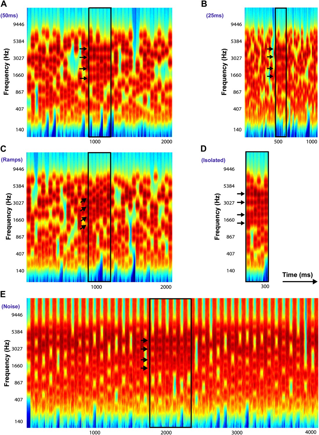
Examples of Stochastic Figure-Ground stimuli.
All stimuli in this example contain four identical frequency components (only for illustrative purposes: these were selected randomly in the experiments) with Fcoh = 1016.7 Hz, 2033.4 Hz, 3046.7 Hz, and 4066.8 Hz repeated over 6 chords and indicated by the black arrows. The figure is bound by a black rectangle in each stimulus. (A) Chord duration of 50 ms: stimulus comprises of 40 consecutive chords each of duration 50 ms with a total duration of 2000 ms. (B) Chord duration of 25 ms: stimulus comprises of 40 consecutive chords each of duration 25 ms with a total duration of 1000 ms. (C) Ramped figures: stimulus comprises of 40 consecutive chords each of duration 50 ms each (like A) but the frequency components comprising the figure increase in frequency in steps of 2*I or 5*I, where I = 1/24th of an octave, represents the resolution of the frequency pool. (D) Isolated figures: stimulus comprises only of the ‘figure present’ portion without any chords preceding or following the figure. The duration of the stimulus is given by the number of chords. (E) Chords interrupted by noise: stimulus comprises of 40 consecutive chords alternating with 40 chords comprising of loud, masking broadband white noise, each 50 ms in duration. In experiment 6b, the duration of the noise was varied from 100 ms to 500 ms (see ‘Materials and methods’).
Figure 2

Behavioral performance in the basic and figure identification task.
The d′ for experiments 1 (A; ‘chord duration of 50 ms’; n = 9) and 2 (B; ‘figure identification’; n = 9) are plotted on the ordinate and the duration of the figure (in terms of number of 50 ms long chords) is shown along the abscissa. The coherence of the different stimuli in experiment 1 is color coded according to the legend (inset) while the coherence in experiment 2 was fixed and equal to six. The AXB figure identification task was different from the single interval alternative forced choice experiments: listeners were required to discriminate a stimulus with an ‘odd’ figure from two other stimuli with identical figure components. Error bars signify one standard error of the mean (SEM).
Figure 3 with 1 supplement

Temporal coherence modeling of SFG stimuli.
The protocol for temporal coherence analysis is demonstrated here for experiment 5. The procedure was identical for modeling the other experiments. A stimulus containing a figure (here with coherence = 4) as indicated by the arrows (A) and another, background only (figure absent) stimulus (B) was applied as input to the temporal coherence model. The model performs multidimensional feature analysis at the level of the auditory cortex followed by temporal coherence analysis which generates a coherence matrix for each stimulus as shown in C and D respectively. The coherence matrix for the stimulus with figure present contains significantly higher cross-correlation values (off the diagonal; enclosed in white square) between the channels comprising repeating frequencies as indicated by the two orthogonal sets of white arrows in C. A magnified plot of the coherence matrix for the figure stimulus is shown in E where the cross-correlation peaks are highlighted in white boxes. The strength of the cross-correlation is indicated by the heat map next to each figure. The stimulus without a figure, that is, which does not contain any repeating frequencies, does not contain significant cross-correlations. This process is repeated for 500 iterations (Niter) for all combinations of coherence and duration. The differences between these two coherence matrices were quantified by computing the maximum cross-correlation for each set of coherence matrices for the figure and the ground stimuli respectively. Temporal coherence was calculated as the difference between the average maxima for the figure and the ground stimuli respectively. The resultant model response is shown for each combination of coherence and duration in F.
Figure 3—Figure supplement 1
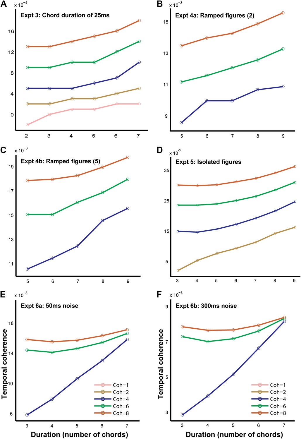
Temporal coherence models for other SFG stimuli.
The output of the temporal coherence modeling procedure is shown for the remaining psychophysical experiments: (A) experiment 2 with 25 ms chords modeled at a rate of 40 Hz; (B, C) experiments 4a and 4b with ramped figures with step size of 2 and 5 respectively modeled at a rate of 10 Hz; (D) experiment 5 with isolated 50 ms chords modeled at a rate of 20 Hz; (E, F) experiments 6a and 6b with chords interrupted by noise of duration 50 ms and 300 ms modeled at 20 Hz and 3.33 Hz respectively.
Figure 4
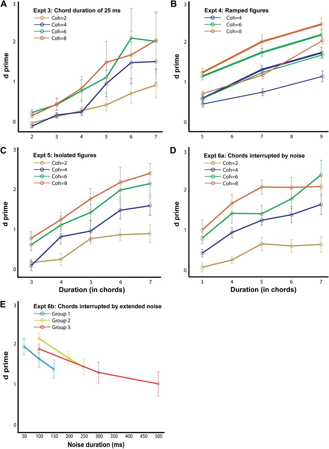
Behavioral performance in the psychophysics experiments.
The d′ for experiment 3, 4a (thick lines; ramp step = 2), 4b (thin lines, ramp step = 5), 5, 6a and 6b are shown here, as labeled in each figure (n = 10 for all conditions). The abscissa represents the duration of the figure (A–D) and the duration of the masking noise in E. Note that the maximum duration value in experiments 4a and 4b is larger (9 chords) than in the other experiments. Error bars signify one SEM.
Download links
A two-part list of links to download the article, or parts of the article, in various formats.
Downloads (link to download the article as PDF)
Open citations (links to open the citations from this article in various online reference manager services)
Cite this article (links to download the citations from this article in formats compatible with various reference manager tools)
Segregation of complex acoustic scenes based on temporal coherence
eLife 2:e00699.
https://doi.org/10.7554/eLife.00699


