A diversity of localized timescales in network activity
- Yale University, United States
- Jacobs University Bremen, Germany
- New York University, United States
Figures
Figure 1
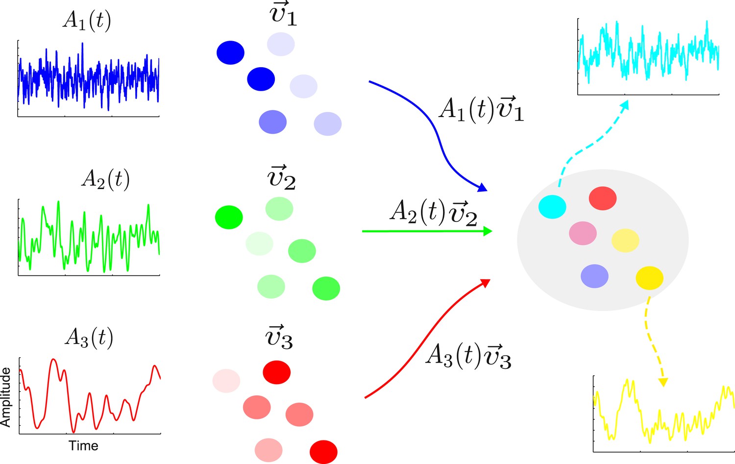
The activity of a linear network can be decomposed into contributions from a set of eigenvectors.
On the right is shown a sample network along with the activity of two nodes (cyan and yellow). The activity of this network is the combination of a set of eigenvectors whose spatial distributions are shown in blue, green and red on the left. The nodes are colored according to the contributions of the various eigenvectors. Each eigenvector has an amplitude that varies in time with a single timescale given by the corresponding eigenvalue; here the blue, green and red eigenvectors have a fast, intermediate and slow timescale, respectively. The cyan node is primarily a combination of the blue and green eigenvectors; hence its activity is dominated by a combination of the blue and green amplitudes and it shows a fast and an intermediate timescale. Similarly, the yellow node has large components in the green and red eigenvectors, therefore its activity reflects the corresponding amplitudes and intermediate and slow timescales.
Figure 2
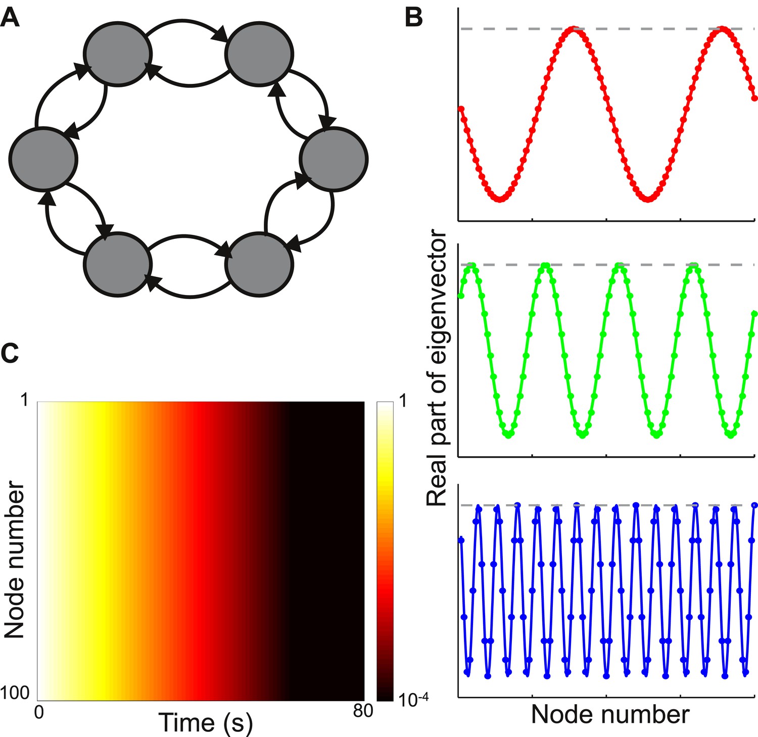
Local connectivity is insufficient to yield localized eigenvectors.
(A) The network consists of 100 nodes, arranged in a ring. Connection strength decays exponentially with distance, with characteristic length of one node, and is sharply localized. The network topology is shown here as a schematic, with six nodes and only nearest-neighbor connections. (B) The eigenvectors are maximally delocalized. Three eigenvectors are shown, and the others are similar. The absolute value of each eigenvector, shown with the gray dashed lines, is the same at all nodes. The real part of each eigenvector, shown in color, oscillates with a different frequency for each eigenvector. (C) Dynamical response of the network to an input pulse, shown on a logarithmic scale. All nodes show similar response timescales.
Figure 3 with 1 supplement

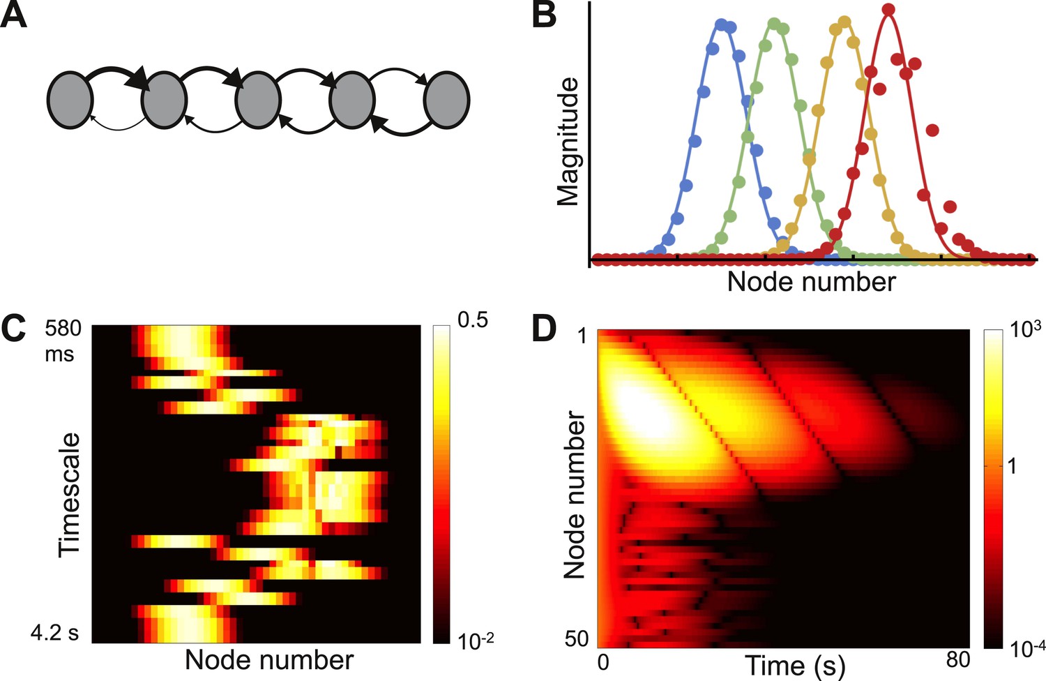
Localized eigenvectors in a network with a gradient of local connectivity.
(A) The network is a chain of 100 nodes. Network topology is shown as a schematic with a subset of nodes and only nearest-neighbor connections. The plot above the chain shows the connectivity profile, highlighting the exponential decay and the asymmetry between feedforward and feedback connections. Self-coupling increases along the chain, as shown by the grayscale gradient. (B) Sample eigenvectors (filled circles) in a network with a weak gradient of self-coupling, so that localized and delocalized eigenvectors coexist. Localized eigenvectors are described by Gaussians, and predictions from Equation 4 are shown as solid lines. Eigenvectors are normalized by maximum value. The network is described by Equation 3, with μ0 = −1.9, Δr = 0.0015, μf = 0.2, μb= 0.1 and lc = 4. (C) Sample eigenvectors (filled circles) along with predictions (solid lines) in a network with a strong gradient, so that all eigenvectors are localized. Network parameters are the same as B, except Δr = 0.01. (D) Heat map of eigenvectors from network in (C) on logarithmic scale. Eigenvectors are along rows, arranged by increasing decay time. All are localized, and eigenvectors with longer timescales are localized further down in the chain. Edge effects cause the Gaussian shape to break down at the end of the chain, but eigenvectors are still localized at the boundary. (E) Dynamical response of the network in (C) to an input pulse. Nodes early in the chain show responses that decay away rapidly, while those further in the chain show more persistent responses.
Figure 3—figure supplement 1
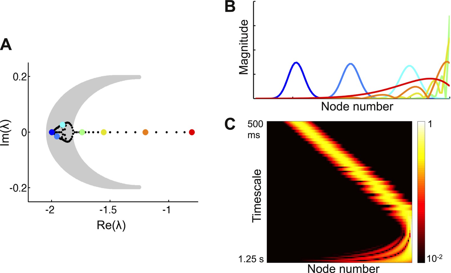
Co-existence of localized and delocalized eigenvectors in a network with a weak gradient of local connectivity.
(A) Left panel: eigenvalues of the network (filled circles) along with the region of the complex plane in which α2 > 0 (gray shaded region). Eigenvectors corresponding to eigenvalues within this region are predicted to be localized. (B) Eigenvectors corresponding to the colored eigenvalues in panel A. Eigenvalues within the gray region correspond to localized eigenvectors. Eigenvectors outside the gray region are progressively more delocalized. Eigenvectors are shown as solid lines for ease of visualization. (C) Heat map of eigenvectors on logarithmic scale. Eigenvectors are along rows, arranged by increasing decay time. The network is described by Equation 3 in the main text, with μ0 = − 1.9, Δr = 0.0015, μf = 0.2, μb = 0.1, and lc = 4.
Figure 4
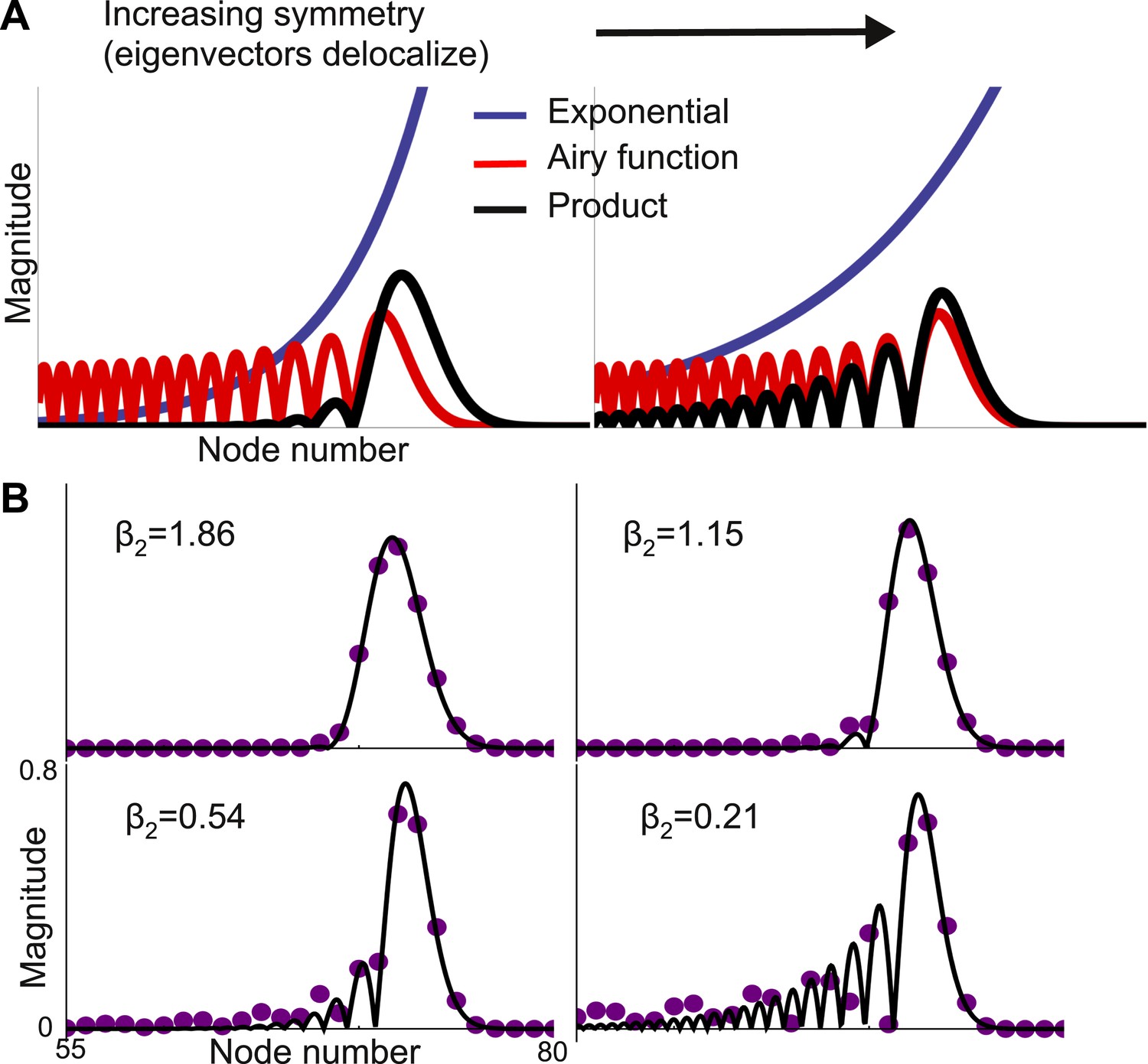
Second-order expansion for partially-delocalized eigenvectors.
Same model with a gradient of local connectivity as in Figure 3. (A) Schematic of the predicted shape. Eigenvectors (black) are the product of an exponential (blue) and an Airy function (red). The constant in the exponential depends on the asymmetry between feedback (μb) and feedforward (μf) strengths. In the left panel, μf − μb is large and the product is well described by a Gaussian. In the right panel, μf − μb is small and the exponential is shallow enough that the product is somewhat delocalized. (B) Analytically predicted eigenvector shapes (solid lines) compared to numerical simulations (filled circles) for four values of μb. For each value of μb one representative eigenvector is shown. As μb approaches μf, eigenvectors start to delocalize but, as per Equation 4, the maximum peak is sharper. β2 is the steepness of the exponential (Equation 5). The network is described by Equation 3 with μ0 = −1.9, Δr = 0.01, μf = 0.2, and lc = 4. μb = 0.125, 0.15, 0.175, and 0.19.
Figure 5
Localized eigenvectors in a network with a gradient of connectivity range.
(A) The network consists of a chain of 50 identical nodes, shown here by a schematic. Spatial length of feedforward connections (from earlier to later nodes) decreases along the chain while the spatial length of feedback connections (from later to earlier nodes) increases along the chain. The network is described by Equation 7, with μ0 = −1.05, μf = 5, μb = 0.5, f0 = 0.2, f1 = 0.12, b0 = 6, b1 = 0.11. Normally-distributed randomness of standard deviation σ = 10−5 is added to all connections. (B) Five sample eigenvectors, with numerical simulations (filled circles) well fitted by the analytical predictions (solid lines). Note the effect of added randomness on the rightmost eigenvector. (C) Heat map of eigenvectors on logarithmic scale. Rows correspond to eigenvectors, arranged by increasing decay time. All eigenvectors are localized, but timescales are not monotonically related to eigenvector position. (D) Dynamical response of the network to an input pulse. Long timescales are localized to nodes early in the network while nodes later in the network show intermediate timescales.
Figure 6
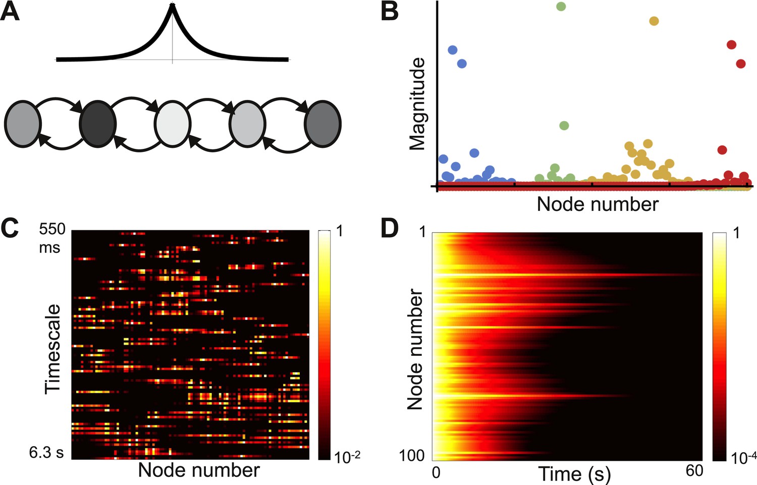
Localized eigenvectors in a network with random self-coupling.
(A) The network consists of 100 nodes arranged in a chain. The plot above the chain shows the connectivity profile. Self-coupling is random, as indicated by the shading. The network is described by Equation 8 with μ0 = −1, μc = 0.05, lc = 4, σ = 0.33. (B) Four eigenvectors are shown, localized to different parts of the network. Note the diversity of profiles. (C) Heat map of eigenvectors on logarithmic scale. Rows correspond to eigenvectors, arranged by increasing decay time. All eigenvectors are localized, though the extent of localization (the eigenvector width) varies; and there is no relationship between the timescale of an eigenvector and its spatial location in the network. (D) Dynamical response of the network to an input pulse. Note that the diversity of dynamical responses is more limited, and bears no relationship to spatial location.
Figure 7
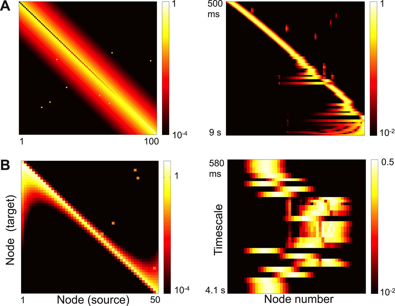
Strong long-range connections can delocalize a subset of eigenvectors.
(A) Left panel: connectivity of the network in Figure 3 with long-range connections of strength 0.05 added between 10% of the nodes. The gradient of self-coupling is shown along the diagonal on another scale, for clarity. Right panel: eigenvectors shown as in panel C of Figure 3. (B) Left panel: connectivity of the network in Figure 5 with long-range connections of strength 0.05 added between 10% of the nodes. Right panel: eigenvectors shown as in panel C of Figure 5.
Additional files
-
Supplementary file 1
Mathematical appendix.
- https://doi.org/10.7554/eLife.01239.011
Download links
A two-part list of links to download the article, or parts of the article, in various formats.
Downloads (link to download the article as PDF)
Open citations (links to open the citations from this article in various online reference manager services)
Cite this article (links to download the citations from this article in formats compatible with various reference manager tools)
A diversity of localized timescales in network activity
eLife 3:e01239.
https://doi.org/10.7554/eLife.01239


