Decoding neural responses to temporal cues for sound localization
Figures
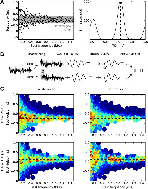
Overview of model.
(A) The distribution of best delay vs best frequency for cells in the guinea pig model (left), with the physiological range of ITDs shown in gray, and a sample tuning curve (right). (B) Illustration of the model: a sound source is filtered via position-dependent HRTFs to give left and right channels. For each best frequency on each channel, the signal undergoes cochlear filtering using gammatone filters. An internal delay is added, and the two channels are combined and sent to a binaural neuron model that produces Poisson distributed spikes. (C) The response of the cells to sounds at two different ITDs (rows) for white noise (left column) and a natural sound (right column). The ITD is indicated by the black dashed line. Each cell is surrounded by a disc with a color indicating the response of that neuron (hot colors corresponding to strong responses). When two or more discs overlap, each point is colored according to the closest cell. The strongest responses lie along the line of the ITD.
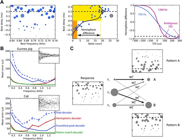
Decoders in single frequency bands.
(A) Peak and hemispheric decoders. Left: response of binaural neurons to sound at ITD = 0.2 ms (dashed line), in a narrow frequency band. The size of points is proportionate to spike count, and the crossed point corresponds to the highest spike count. Middle: the same cell responses are displayed as best delay vs spike count (note the different horizontal axis). The solid black line is the Gaussian smoothed spike count, whose peak (circle) is the ITD estimate. The maximally responsive neuron is also indicated with a circle for comparison. The yellow and orange bars give the mean response of neurons with positive and negative best delays, respectively, from which the normalized hemispheric difference is computed. Right: the hemispheric difference as a function of ITD at 700 Hz (blue) and 1.3 kHz (purple). At 1.3 kHz, the difference shown by the dashed line gives an ambiguous estimate of the ITD. (B) Mean error for the guinea pig and cat, for the peak (blue, dashed), smoothed peak (blue, solid), hemispheric (red), and pattern match (green) decoders. The distribution of BD vs BF is shown in the inset. (C) Illustration of the pattern match decoder and a neural circuit that implements it. The response (left) is compared to two patterns A and B, corresponding to two different ITDs (right). Each response neuron is connected to a pattern-sensitive neuron with weights proportional to the stored response of each pattern. When the weights match the responses, the output of the pattern-sensitive neuron is strongest.
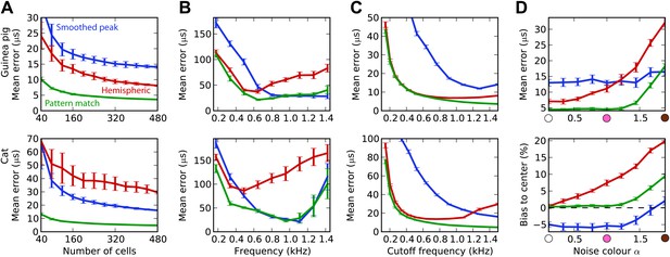
Integration across frequencies.
(A) Mean error in estimating ITD for white noise using the smoothed peak (blue), hemispheric (red), and pattern match (green) decoders, as a function of the number of binaural cells. Training and testing of the decoders are both performed using white noise. (B) Mean error as a function of frequency band when decoders are trained on white noise but tested on band-pass noise centered at the given frequency. Notice the different vertical scale between (A and B). (C) Performance when cells with a frequency above the cutoff are discarded. (D) Mean error and bias to center in the decoders for guinea pig (with a maximum frequency of 1.2 kHz) when trained on white noise and tested on colored noise.
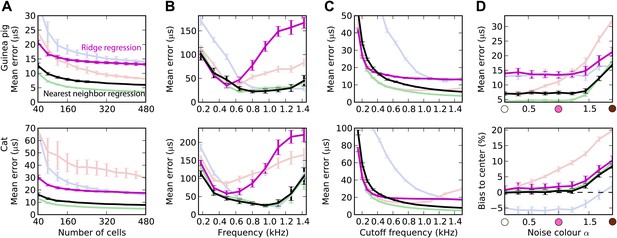
Comparison with standard machine learning decoders.
As for Figure 3, except that the main decoders are shown in light colors, and there are two additional decoders: ridge regression (magenta) and nearest neighbor regression (black).
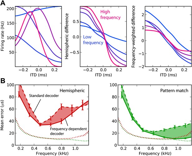
Frequency-dependent improvements.
(A) Comparing hemispheric differences across frequency channels. In each plot, color indicates frequency with red being high frequency and blue being low frequency. Left: tuning curves for a few binaural neurons. Middle: hemispheric difference (L − R)/(L + R). Right: frequency-dependent hemispheric difference (1/f) (L − R)/(L + R). (B) Mean error as a function of frequency band in the guinea pig model, for hemispheric (red) and pattern match (green) decoders (dashed lines), and frequency-dependent hemispheric and pattern match (solid) decoders. The shaded regions show the difference between the simple and frequency-dependent versions. The dotted lines show the mean error for band-pass noise if the decoder is trained and tested on the same frequency band, as shown in Figure 2B (guinea pig). This represents the lower bound for the error.
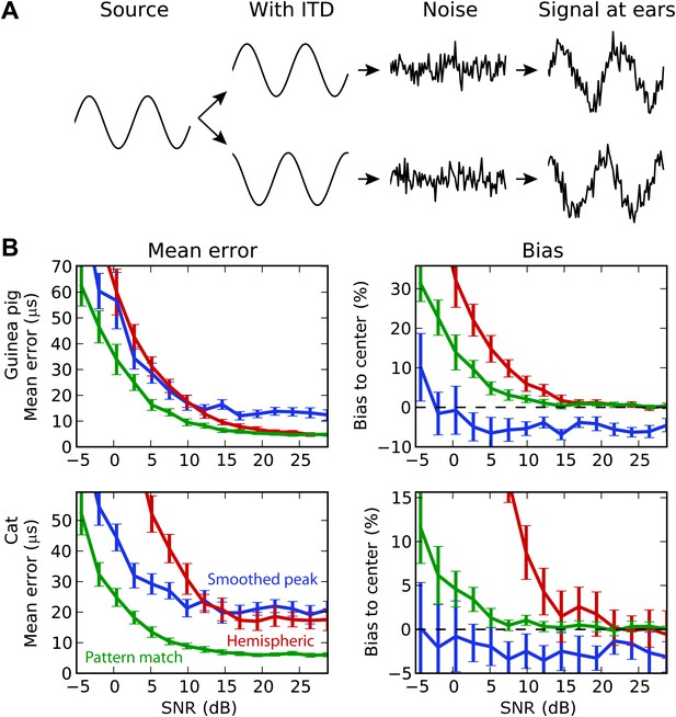
Background acoustic noise.
(A) Illustration of protocol: a binaural sound is presented with a given ITD, with independent white noise added to the two channels. (B) Mean error (left column) and central bias (right column) at different signal to noise levels. Decoders are smoothed peak (blue), hemispheric (red), and pattern match (green).
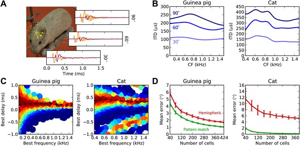
Realistic head-related transfer functions.
(A) Photograph of stuffed guinea pig used for HRTF recordings, and three pairs of left/right ear impulse responses corresponding to the directions marked on the photograph. (B) Frequency dependence of ITD for the three azimuths shown in panel (A), in guinea pig and cat HRTFs. (C) Mean response of the model to white noise stimuli at the same azimuth (90°) for both animals, the frequency-dependent ITD curve is shown for this azimuth (dashed). (D) Performance of the model as a function of the number of cells for hemispheric (red) and pattern match (green) decoders.
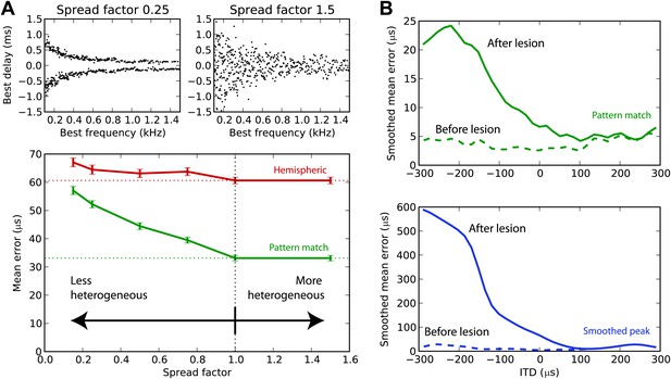
Effect of heterogeneity and lesions.
(A) Mean error for the hemispheric (red) and pattern match (green) decoders in the guinea pig model, depending on the spread of the best delays, for white noise presented with acoustic noise (SNR between −5 and 5 dB, no HRTF filtering). For every frequency, the standard deviation of BDs is multiplied by the spread factor: lower than 1 denotes less heterogeneous than the original distribution (top left), greater than 1 denotes more heterogeneous (top right). Dashed lines represent the estimation error for the original distribution. (B) Mean error for the pattern match (green) and smooth peak (blue) decoders before (dashed) and after (solid) lesioning one hemisphere in the guinea pig, as a function of presented ITD. The model is retrained after lesioning. The error curves are Gaussian smoothed to reduce noise and improve readability.
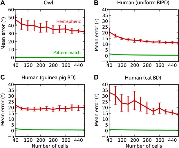
Humans and owls.
(A) Mean error for the pattern match (green) and hemispheric (red) decoders for the barn owl model, with sounds presented through measured HRTFs. (B) Performance in the human model with uniformly distributed best interaural phase differences. (C) Performance in the human model with best delays distributed as in the guinea pig model. (D) Performance in the human model with best delays distributed as in the cat model.
Tables
Summary of animal models
| Name | ITD source | ITD range, μs | Best delays (BD) | Best frequencies (BF) | α | β | k |
|---|---|---|---|---|---|---|---|
| Guinea pig | Artificial | ± 300 | Measured | 100–1500 Hz | 0.35 | 4.0 | 8 |
| Guinea pig | HRTF | ± 250 | Measured | 100–1500 Hz | 0.35 | 4.0 | 8 |
| Cat | Artificial | ± 400 | Measured | 100–1500 Hz | 0.37 | 5.0 | 4 |
| Cat | HRTF | ± 450 | Measured | 400–1500 Hz | 0.37 | 5.0 | 4 |
| Human | HRTF | ± 950 | Uniform within π-limit | 100–1500 Hz | 0.37 | 5.0 | 4 |
| Human | HRTF | ± 950 | Guinea pig distribution | 100–1500 Hz | 0.37 | 5.0 | 4 |
| Human | HRTF | ± 950 | Cat distribution | 100–1500 Hz | 0.37 | 5.0 | 4 |
| Owl | HRTF | ± 260 | Measured | 2–8 kHz | 0.50 | 4.3 | 2 |


