Fast transient networks in spontaneous human brain activity
- University of Oxford, United Kingdom
- University of Nottingham, United Kingdom
- Oxford University, United Kingdom
- University College London, United Kingdom
Figures
Figure 1
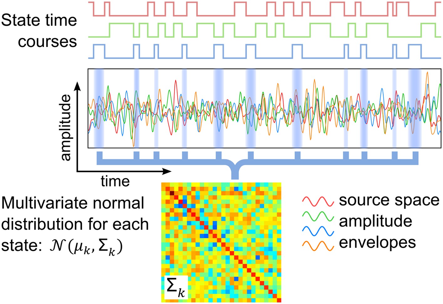
Schematic of the HMM outputs.
An HMM with K states is inferred from band-limited amplitude envelopes of source reconstructed MEG data. Each state is characterized by a multivariate normal distribution (defined by means μk and covariance matrix Σk) and a state time course, which is a binary sequence that indicates the points in time at which the state is active.
Figure 2 with 2 supplements
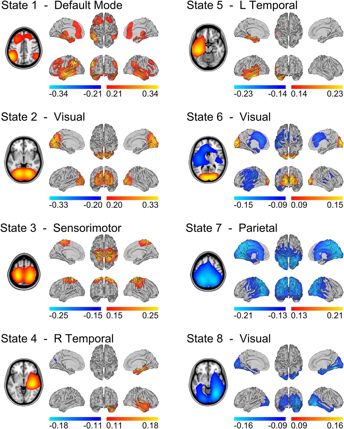
State specific changes in band-limited amplitude.
An 8 state HMM was inferred from temporally concatenated band-limited amplitude time courses (concatenated over nine subjects, 10 min each). The volumes and surface renderings show the partial correlation of each state time course with the envelope data at each voxel. The correlation values have been thresholded between 60% and 100% of the maximum correlation for each state and the color maps represent these ranges. Red/yellow and blue colors indicate positive and negative correlations respectively. See also Figure 2—figure supplement 1 for equivalent results from HMMs inferred with 4–14 states.
Figure 2—figure supplement 1
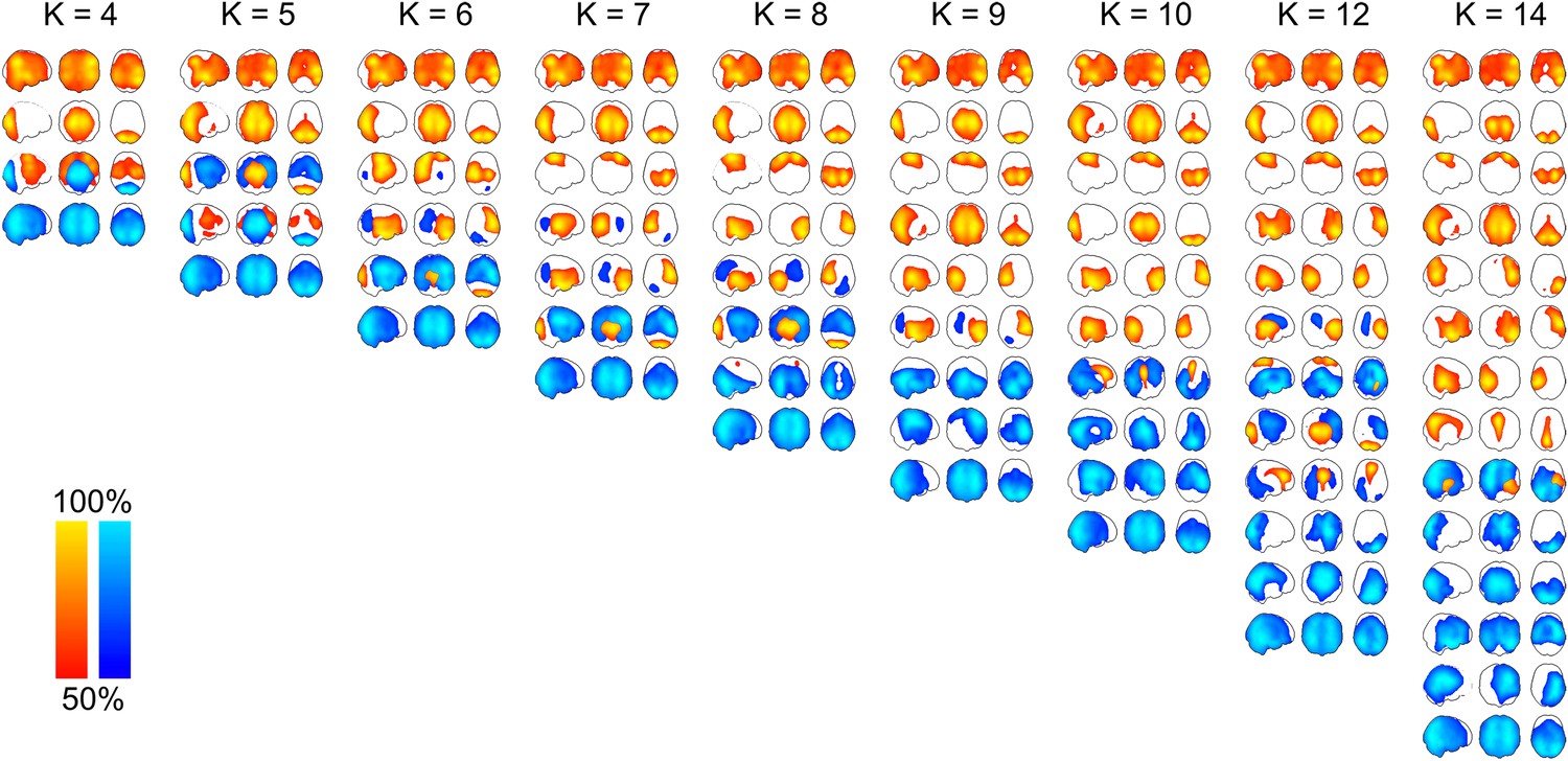
Maximum intensity projection maps showing the partial correlation computed between each state time course and the envelope data for a k state HMM for k = 4 to k = 14.
Increasing the number of states did not change the topographies of the most prominent RSN-like states nor did it reveal any new RSN-like topographies that were distinct from those inferred with 8 states, but rather resulted in the splitting of states into multiple similar maps. This suggests that there is no advantage to using more than 8 states for the purpose of identifying states corresponding to known RSNs. In fact, it could be argued that fewer than 8 states are required for this purpose.
Figure 2—figure supplement 2
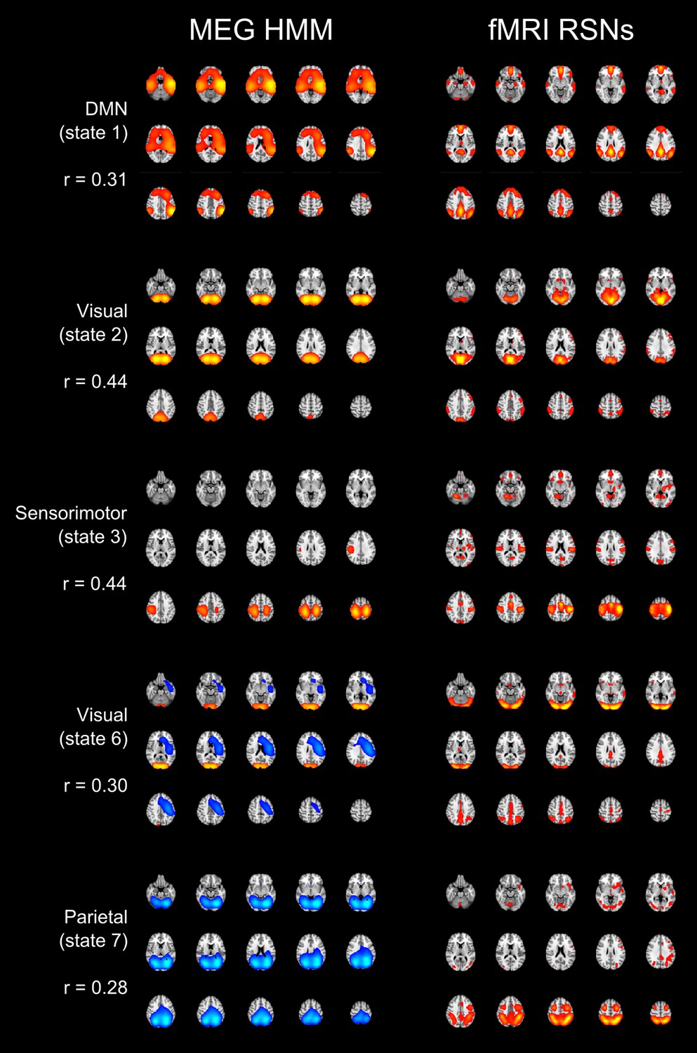
Spatial maps of five of the inferred states alongside a matched RSN derived from application of spatial ICA to resting state fMRI data (Smith et al., 2009).
For each HMM–RSN pair, the spatial correlation is shown alongside the maps.
Figure 3 with 1 supplement

Temporal characteristics of the HMM states.
(A) State time courses showing the most likely state at each time point for the first 10 s of data. (B) Fractional occupancy for each inferred state showing the mean and s.e.m. over subjects. The asterisks denote that the fractional occupancy of a state differs significantly from the other states. (C) Life times, and (D) interval lengths for each inferred state. The filled areas in (C) and (D) represent the distribution of values and the black crosses show the mean. (E) Fractional occupancy of each state as a function of time over all subjects, derived by averaging each state time course within a 10-s sliding window (75% overlap between adjacent windows). See also Figure 3—figure supplement 1 for a description of how these statistics vary when the HMM is inferred with 4–14 states.
Figure 3—figure supplement 1
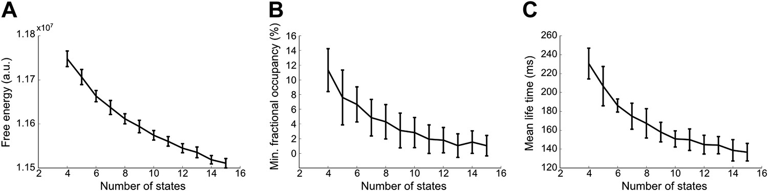
Effect of number of states on (A) model evidence, approximated by the negative of the free energy, (B) minimum fractional occupancy and (C) mean life time, computed over all inferred states and 50 realizations of each HMM inference.
Error bars show the mean and s.e.m. over all subjects. The free energy monotonically increases up to 15 states suggesting that the Bayes-optimal model may require an even higher number of states (A). However, a larger number of states result in a decrease in minimum fractional occupancy (B). This may provide a more meaningful metric since a sufficient amount of data is required for reliable estimation of the covariance matrix. Increasing the number of states also has an effect on the mean life times of the inferred states. Varying the number of states from 4 to 15 results in mean lifetimes decreasing from 230 ms to 140 ms (C). This suggests that the splitting of states that arises from increasing the number of states does not result in states with fewer occurrences, but rather a splitting into shorter-lived events.
Figure 4 with 1 supplement
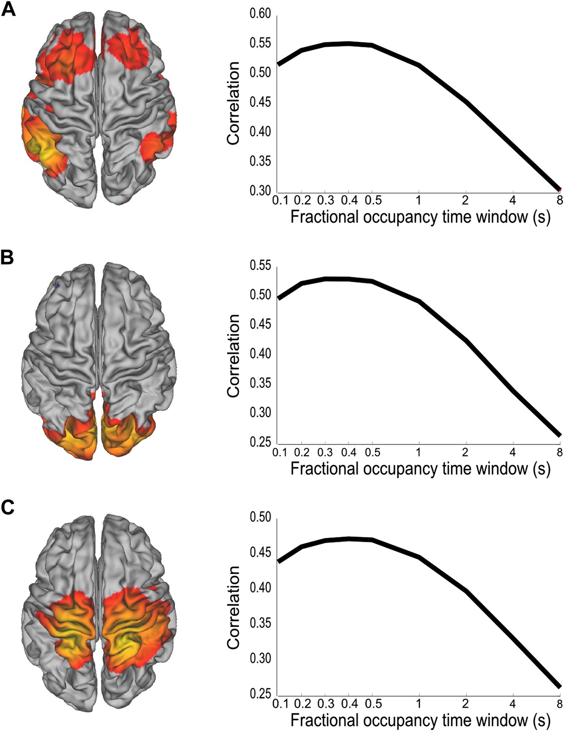
Analysis of the time scales that best reflect within-network envelope fluctuations.
Partial correlation maps and fractional occupancy time window dependency are shown for (A) DMN, (B) visual network and (C) sensorimotor network. The fractional occupancy time window dependency was computed by fitting a GLM to the amplitude envelope at the voxel with highest correlation with the state time course with the fractional occupancy (computed within different time windows) as a single regressor. See also Figure 4—figure supplement 1 for a control analysis with surrogate data.
Figure 4—figure supplement 1
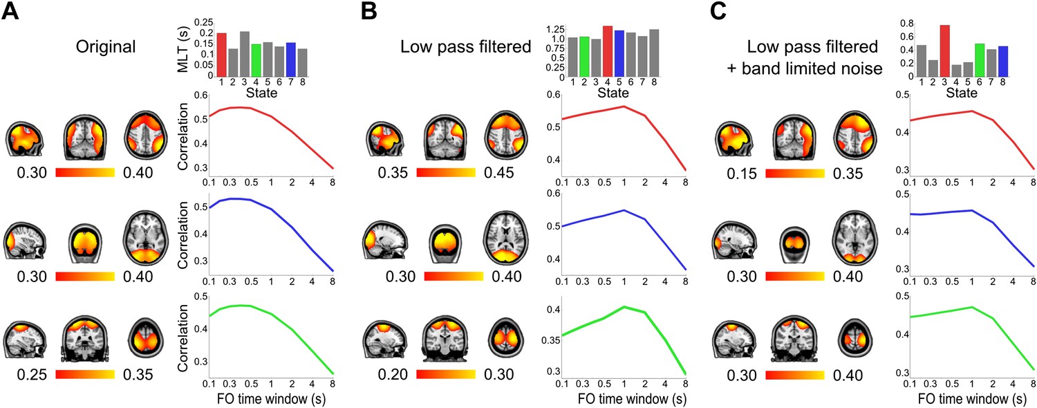
Control analysis of the time scales that best reflect within-network envelope fluctuations.
Correlation maps, mean life times, and fractional occupancy time window dependency for 8 state HMMs inferred from (A) the original group-concatenated envelopes, (B) these envelopes low pass filtered below 0.5 Hz and (C) these low pass filtered envelopes with uncorrelated Gaussian noise added. Results are shown for the default mode network (top/red), visual network (middle/blue) and sensorimotor network (bottom/green). The correlation maps were computed by fitting a GLM to the data with the state time courses for all states as regressors. The fractional occupancy time window dependency was computed by fitting a GLM to the data with the fractional occupancy time course (computed within different time windows) as a single regressor.
Figure 5
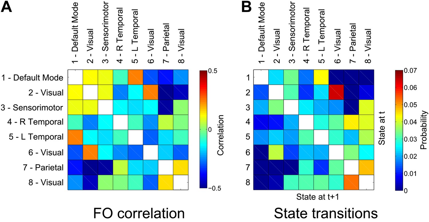
Relationship between states.
(A) Correlation matrix between the fractional occupancy time courses of each state. Positive correlations between a pair of states indicate that the two states are visited more frequently during similar periods of time. (B) State transition matrix for the group HMM. The matrix shows the probabilities of transitioning to any particular state given the current state. The probability of remaining in the same state has been excluded from each matrix (shown in white).
Figure 6
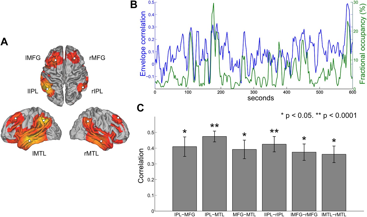
Comparison between HMM state occupancy and sliding window envelope correlation.
(A) Six nodes identified from the DMN state (rIPL, lIPL, rMFG, lMFG, rMTG, lMTG). (B) Time courses of rIPL-rMFG envelope correlation (blue) and DMN state fractional occupancy (green) for a single subject computed using a 10-s sliding window (75% overlap between adjacent windows). (C) Correlation between the sliding window envelope correlation time course and fractional occupancy time course for each ipsilateral pair (bilaterally homologous pairs from the left and right hemispheres have been averaged together) and each contralateral pair (mean and s.e.m. over subjects).
Author response image 1

Power spectra for each state.
The (pre-enveloped) data for each subject and at each voxel were decomposed into a time-frequency representation using Morlet wavelets (Morlet factor = 6). The magnitude of the transformed data was averaged both inside and outside of the state, using the time points indexed by the state time courses, resulting in an inside-state and outside-state power spectrum at each voxel. Weighted averages of these spectra were computed using the spatial maps in Figure 2. The red and blue plots show the averaged power spectra computed inside and outside the state respectively. The shaded region shows the s.e.m. over all subjects and the circles show the frequencies corresponding to each wavelet scale used.
Author response image 2
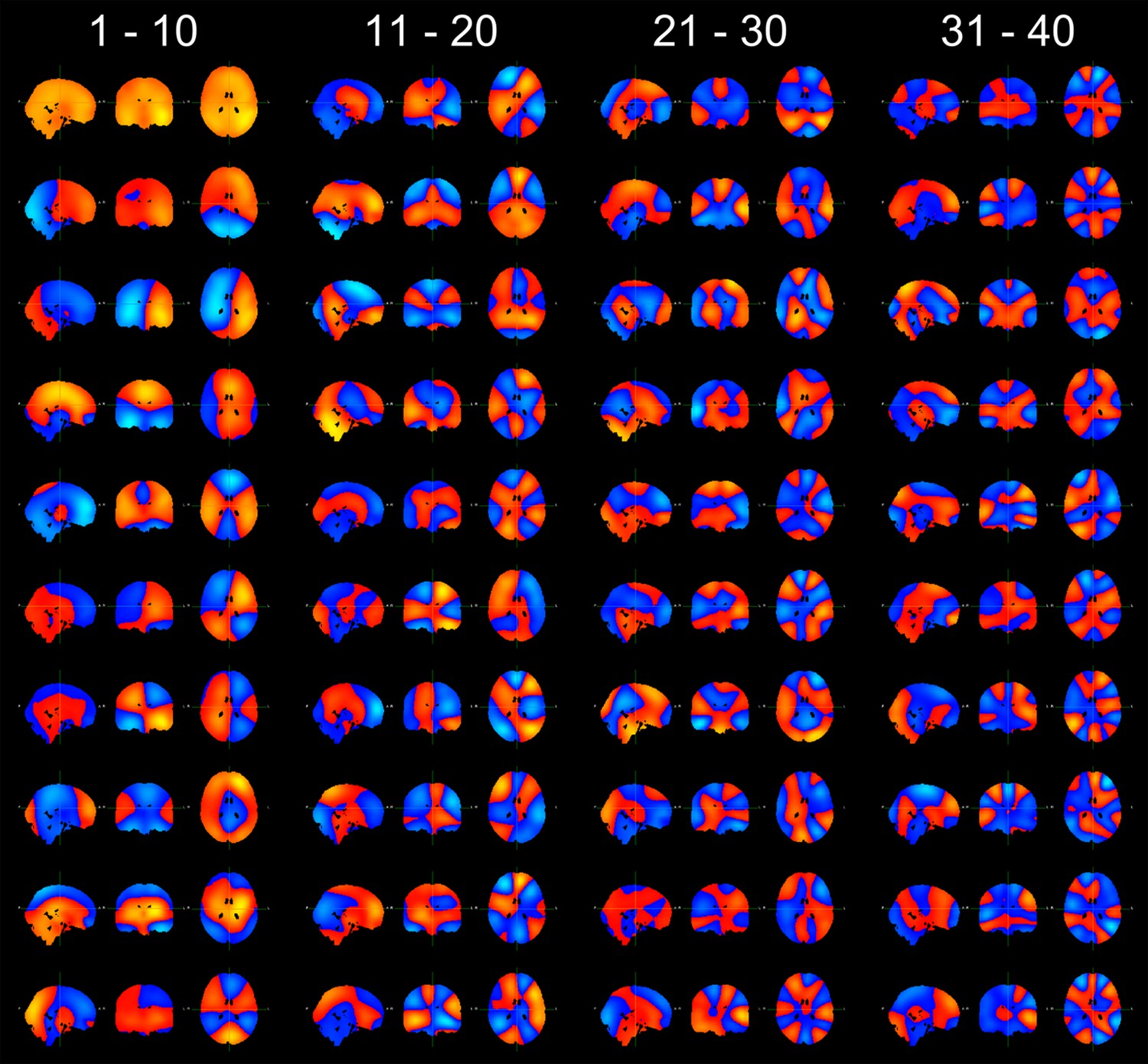
Spatial maps showing (A) pre- and (B) post- PCA variance of the 4-30 Hz band limited envelopes averaged over subjects. The maps in (C) show the average of the unthresholded states’ spatial maps (the sign was ignored when taking the average, to avoid state-specific increases and decreases from cancelling each other out).
Author response image 3
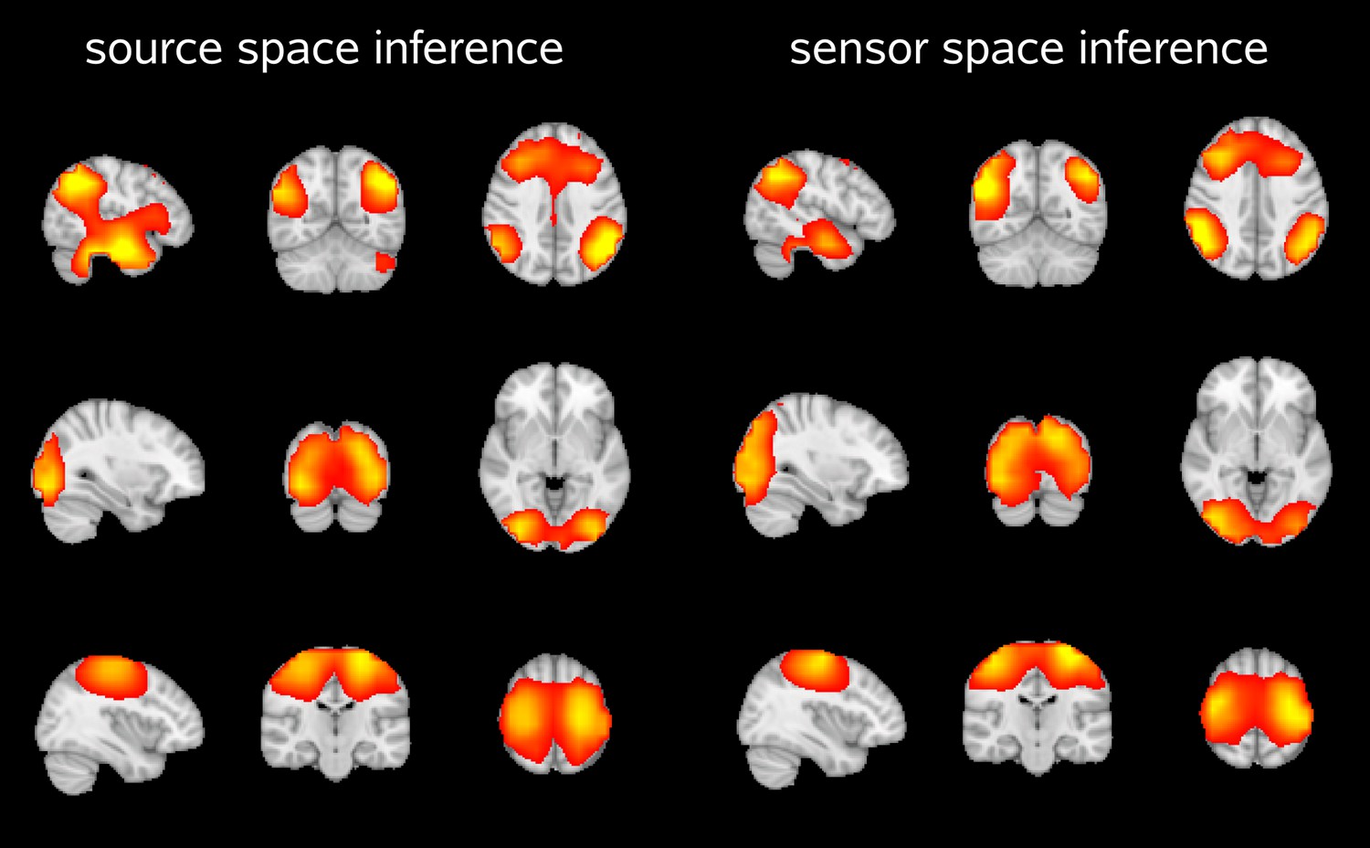
Spatial maps showing the partial correlation of the source space amplitude envelopes with state time courses of an HMM inferred in source space and sensor space.
Both approaches reveal very similar maps for the default mode network (top), visual network (middle) and sensorimotor network (bottom).
Author response image 4
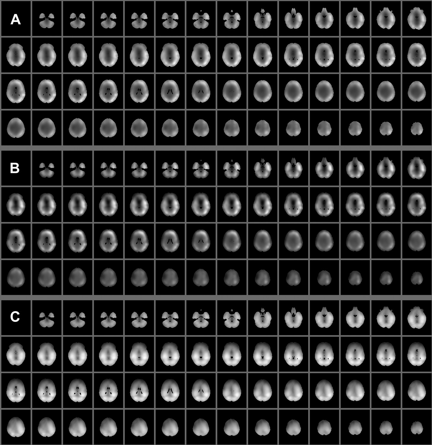
Spatial topographies of the 40 principal components, arranged in order of their variance (top to bottom, left to right).
The cross hairs are positioned at the center of the head (MNI coordinates [0 -18 18]).
Download links
A two-part list of links to download the article, or parts of the article, in various formats.
Downloads (link to download the article as PDF)
Open citations (links to open the citations from this article in various online reference manager services)
Cite this article (links to download the citations from this article in formats compatible with various reference manager tools)
Fast transient networks in spontaneous human brain activity
eLife 3:e01867.
https://doi.org/10.7554/eLife.01867


