Genome-wide mapping in a house mouse hybrid zone reveals hybrid sterility loci and Dobzhansky-Muller interactions
- Max Planck Institute for Evolutionary Biology, Germany
- University of Wisconsin, United States
Figures
Figure 1 with 2 supplements
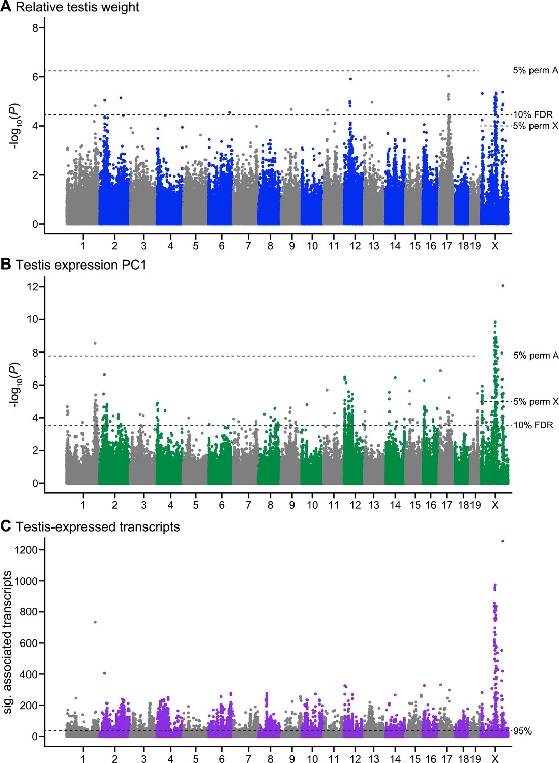
Manhattan plot of GWAS results.
Single SNPs associated with (A) relative testis weight, (B) testis expression principal component 1, and (C) expression of transcripts located on other chromosomes (trans). Dashed lines indicate significance thresholds based on: permutations for autosomes (labeled 5% perm A), permutations for X chromosome (labeled 5% perm X), false discovery rate <0.1 (labeled 10% FDR), and 95th percentile of significant transcript association counts across SNPs (labeled 95%).
-
Figure 1—source data 1
SNPs significantly associated with relative testis weight and/or testis expression PC1 (excel file).
- https://doi.org/10.7554/eLife.02504.006
Figure 1—figure supplement 1
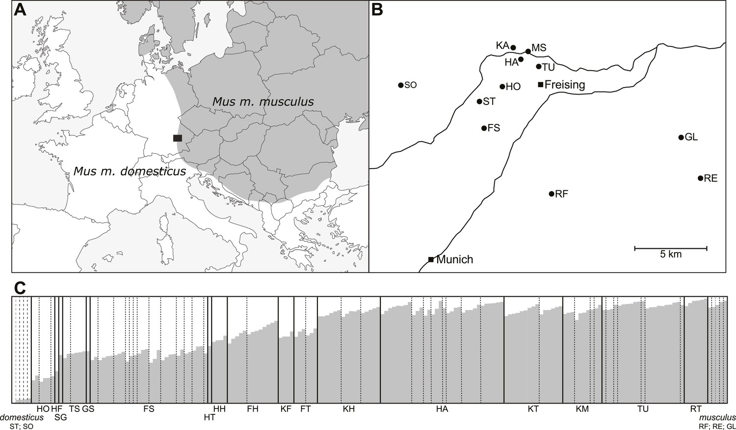
Geographic location of and genetic makeup of mapping population.
(A) Location of sampling area (black box) in European house mouse hybrid zone. (B) Sampling locations for parents of mice in the mapping population. (C) Structure analysis of mapping population. Individuals (vertical bands) are arranged by geographic origin and average percentage alleles from Mus musculus musculus.
Figure 1—figure supplement 2
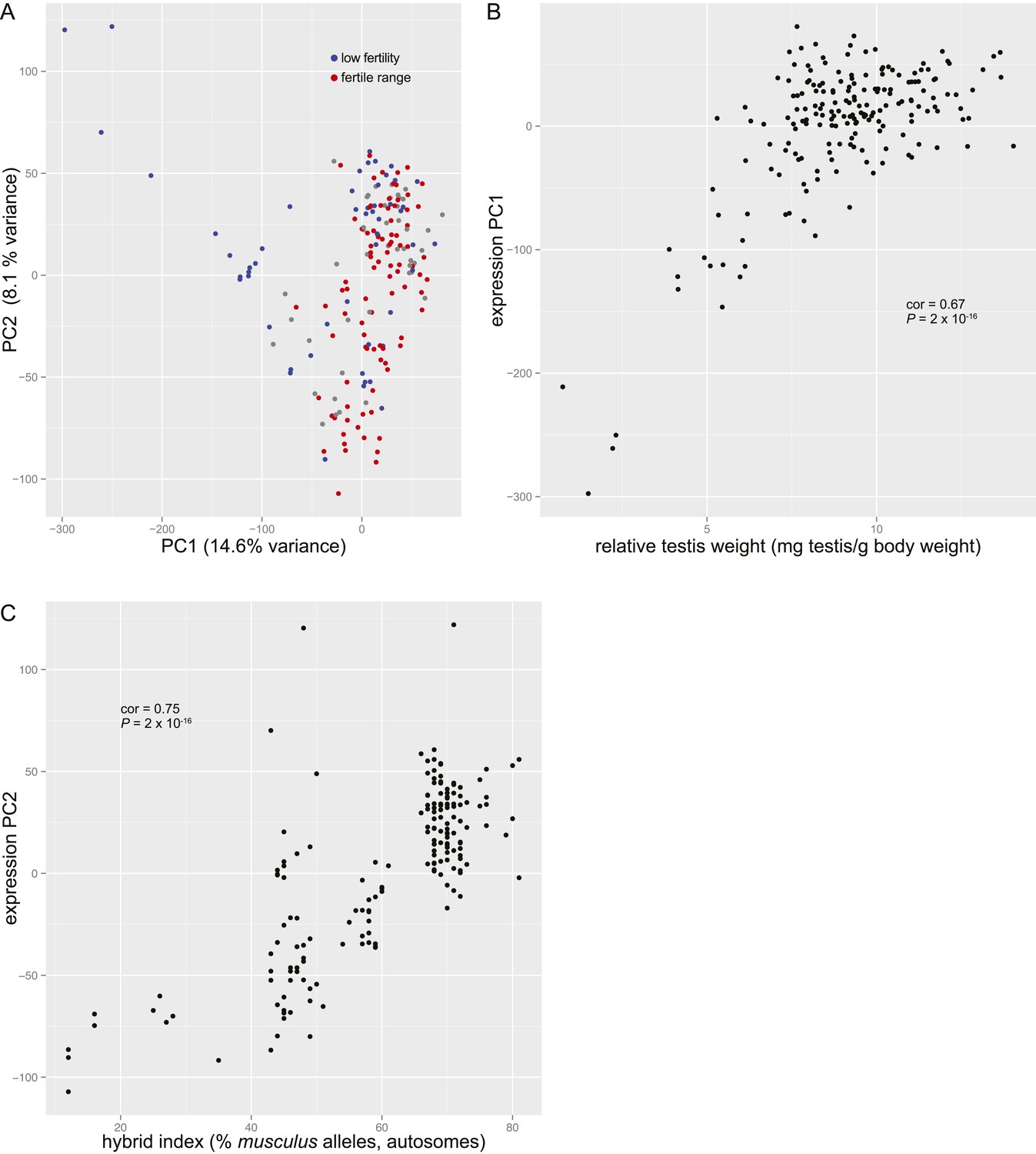
Principal components analysis of genome-wide gene expression in testis.
(A) Plot of principal component 1 (PC1) vs PC2 scores. Individuals with relative testis weight and/or sperm count below the pure subspecies range are indicated in blue (‘low fertility’). Individuals with relative testis weight and sperm count within one standard deviation of the mean in pure subspecies individuals are indicated in red (‘fertile range’). (B) Plot of relative testis weight vs PC1 score. Correlation coefficient (Pearson's) and p value are indicated. (C) Plot of hybrid index (% musculus alleles on autosomes) vs PC2 score. Correlation coefficient (Pearson's) and p value are indicated.
Figure 2 with 1 supplement

Significant GWAS regions and interactions in hybrid zone mice.
Results for (A) relative testis weight and (B) testis expression principal component 1 in hybrid zone mice. In (A) orange and yellow boxes in outer rings (outside grey line) indicate quantitative trait loci (QTL) identified for testis weight and other sterility phenotypes in previous studies (see Table 1 for details). Green boxes indicate significant GWAS regions for relative testis weight. Green lines represent significant genetic interactions between regions; shade and line weight indicate the number of significant pairwise interactions between SNPs for each region pair. In (B) orange boxes in outer rings indicate QTL for testis-related phenotypes (testis weight and seminiferous tubule area) identified in previous studies, yellow boxes indicate QTL for other sterility phenotypes and red boxes indicate trans eQTL hotspots (see Table 2 for details). Green boxes indicate significant GWAS regions for relative testis weight. Purple boxes indicate significant GWAS regions for testis expression PC1. Lines represent significant genetic interactions between regions; color and line weight—as specified in legend—indicate the number of significant pairwise interactions between SNPs for each region pair. Plot generated using circos (Krzywinski et al., 2009).
-
Figure 2—source data 1
Significant genetic interactions (SNP pairs) for relative testis weight (excel file).
- https://doi.org/10.7554/eLife.02504.012
-
Figure 2—source data 2
Significant genetic interactions (SNP pairs) for testis expression PC1 (excel file).
- https://doi.org/10.7554/eLife.02504.013
Figure 2—figure supplement 1

Genetic interactions associated with hybrid sterility in hybrid zone mice and in F2 hybrids.
Orange boxes in outer rings indicate QTL for testis-related phenotypes (testis weight and seminiferous tubule area) identified in previous studies, yellow boxes indicate QTL for other sterility phenotypes, and red boxes indicate trans eQTL hotspots (see Table 2 for details). Green boxes indicate significant GWAS regions for relative testis weight. Purple boxes indicate significant GWAS regions for testis expression PC1. Lines represent significant genetic interactions identified in hybrid zone mice for relative testis weight (in green) and expression PC1 (in purple), which are concordant with genetic interactions identified by mapping expression traits in F2 hybrids (Turner et al., 2014). Plot generated using circos (Krzywinski et al., 2009).
Figure 3
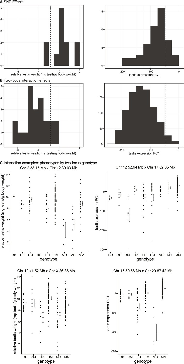
Phenotypic effects of testis-weight loci and interactions.
Histograms showing maximum deviations from the population mean for (A) single SNPs and (B) two-locus interactions. Dashed vertical lines indicate minimum values observed in pure subspecies males. (C) Examples of phenotypic means by two-locus genotype for autosomal–autosomal and X–autosomal interactions. Genotypes are indicated by one letter for each locus: D—homozygous for the domesticus allele, H—heterozygous, M—homozygous musculus.
Figure 4 with 2 supplements
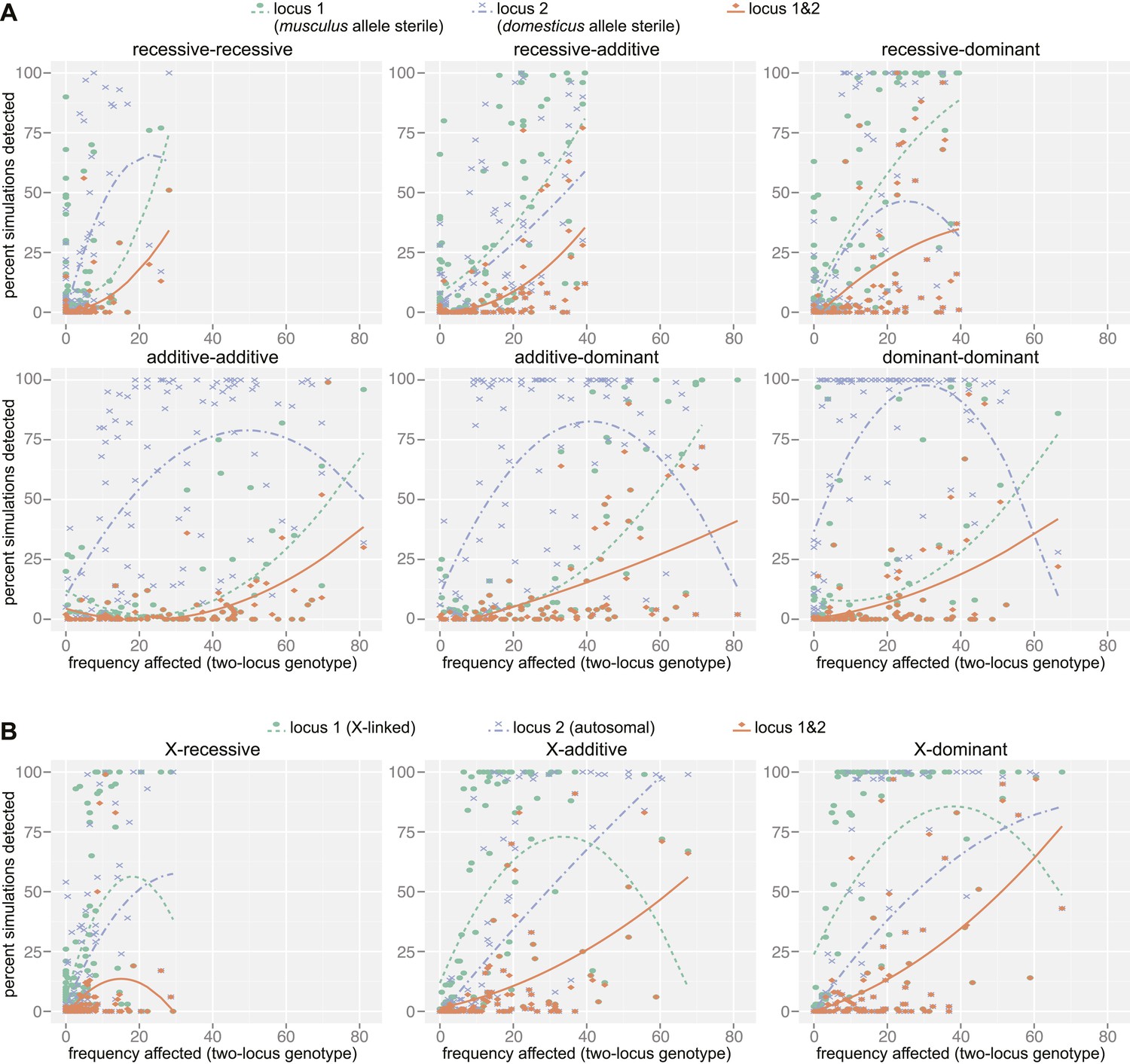
Mapping power in simulations.
Each panel illustrates results from a single genetic architecture model for (A) 100 autosomal–autosomal SNP pairs and (B) 100 X—autosomal SNP pairs. Each point represents the percentage of data sets generated from a single SNP pair in which locus 1 (domesticus sterile allele; green), locus 2 (musculus sterile allele; purple), or both loci (orange) were identified by association mapping (≥1 SNP significant by permutation based threshold within 10 Mb of ‘causal’ SNP). The x axis indicates the percentage of individuals with partial or full sterility phenotypes. Curves were fit using second order polynomials. In (A), locus 1 indicates the SNPs with musculus alleles sterile and locus 2 indicates the SNPs with domesticus alleles sterile. In (B), locus 1 is the X-linked SNP and locus 2 is the autosomal SNP.
-
Figure 4—source data 1
Z scores for simulation models.
- https://doi.org/10.7554/eLife.02504.017
Figure 4—figure supplement 1

Mapping simulation methods.
Schematics of (A) choice of ‘causal’ SNP pairs from the genotype data, (B) phenotype distributions for simulations, (C) generation of simulated phenotype data sets, (D) association mapping. In (B) histogram shows the empirical distribution of relative testis weight in the mapping population, in standard deviation units.
Figure 4—figure supplement 2

Distances of significant SNPs to causal SNP in simulations.
Distributions are shown at two scales for autosomal and X-linked loci.
Tables
Table 1
Genomic regions significantly associated with relative testis weight
| Region*1 | Chr | Position (Mb)† | Length (kb) | Sig. SNPs (5% perm)‡ | No. sign SNPs expression§ | Interactions# | Concordant PC1 region¶ | Concordant sterility loci** | Sterile Allele†† | No. genes (coding) ‡‡ | Candidate Genes§§ |
|---|---|---|---|---|---|---|---|---|---|---|---|
| RTW01 | 1 | 173.30–173.34 | 40.7 | 1 | 1 | 5 | PC03 | d | 3 (3) | ||
| RTW02 | 2 | 33.15 | 2.6 | 1 | 0 | 4 | PC04 | BHZ | m* | 1 (1) | |
| RTW03 | 2 | 129.59–129.65 | 59.8 | 1 | 1 | 2 | PC08 | TWA | d | 2 (1) | |
| RTW04 | 6 | 132.63 | – | 1 | 0 | 0 | – | M | 0 | ||
| RTW05 | 9 | 64.40 | – | 1 | 0 | 3 | – | U | 1 (1) | ||
| RTW06 | 11 | 24.25 | 0.8 | 1 | 1 | 2 | PC26 | BHZ | D | 0 | |
| RTW07 | 12 | 37.16–41.52 | 4364.2 | 4 | 4 | 7 | PC29 | D | 20 (12) | Arl4aEFG | |
| RTW08 | 13 | 51.44 | – | 1 | 0 | 4 | – | TWB | d | 0 | |
| RTW09 | 17 | 56.68–58.44 | 1752.2 | 4 | 2 | 8 | PC43 | SCbinA; TWA; BHZ | M | 42 (39) | Acsbg2E; ClppG; SafbG; Tmem146EG |
| RTW10 | X | 12.17 | – | 1 (1) | 1 | 4 | PC46 | ASHD; eQTLHSC; HTA; SCA | m* | 1 (1) | |
| RTW11 | X | 85.13–98.43 | 13294.3 | 35 (2) | 35 | 3 | PC49 | ASHD; DBTA; eQTLHSC; FERTB; HTA; PBTA; SCB; TASA; TWBD; BHZ | D | 191 (67) | ArEFG; ArxG; Pcyt1bEFG; Tex11EFG; ZfxEFG |
| RTW12 | X | 127.57–134.13 | 6555.5 | 4 (1) | 4 | 2 | PC50 | ASHD; eQTLHSC; shPC1A; SCD; TWD; BHZ | D | 158 (71) | Nxf2G; Taf7lEFG |
-
*
Significant SNPs <10 Mb apart were combined into regions.
-
†
Significant intervals were defined by positions of the most proximal and distal SNPs with LD > 0.9 to a significant SNP.
-
‡
The number of SNPs significant at FDR < 0.1 is reported; number of significant SNPs significant with <0.05 P value in permutations is in parentheses.
-
§
Number of significant SNPs enriched for associations with transcripts expressed on another chromosome (P < 0.05; FDR < 0.1; >30 transcripts).
-
#
Number of regions with significant interactions.
-
¶
Overlapping regions significant for expression PC1 (see Table 2).
-
**
Sterility QTL overlapping or within 10 Mb from A(White et al. 2011), B(Dzur-Gejdosova et al. 2012), C(Turner et al. 2014), D(Good et al. 2008b). Abbreviations for phenotypes: ASH: abnormal sperm head morphology, TW: testis weight, SC: sperm count, shPC1: sperm head shape PC1, eQTLHS: trans eQTL hotspot, FERT: fertility, PBT: proximal bent sperm tail, HT: headless/tailless sperm, DBT: distal bent sperm tail, TAS: total abnormal sperm. BHZ: overlapping candidate regions with evidence from epistasis in the Bavarian hybrid zone transect (Janousek et al. 2012).
-
††
Sterile allele inferred on the basis of frequency of a majority of significant SNPs in pure subspecies samples: D–domesticus; M–musculus; lower-case indicates FST< 0.7 between pure subspecies; * indicates overlapping PC1 region is D sterile; U–nondiagnostic SNP and/or no majority allele.
-
‡‡
Number of genes (protein-coding) overlapping region.
-
§§
Genes with roles in male reproduction on the basis of Emale reproduction gene ontology terms (see ‘Materials and methods’) or phenotypes of knockout models reported in F(Matzuk and Lamb 2008) or GMGI database.
-
Table 1—source data 1
Protein-coding genes in significant relative testis weight regions.
- https://doi.org/10.7554/eLife.02504.004
Table 2
Genomic regions significantly associated with testis expression PC1
| Region* | Chr | Position (Mb)† | Length (kb) | Sig. SNPs (5% perm)‡ | No. sign SNPs expression§ | Interactions# | Concordant RTW region¶ | Concordant sterility loci** | Sterile Allele†† | No. genes (coding) ‡‡ | Candidate Genes§§ |
|---|---|---|---|---|---|---|---|---|---|---|---|
| PC01 | 1 | 8.01–12.72 | 4715.2 | 4 | 4 | 46 | BHZ | U | 40 (18) | Mybl1GH | |
| PC02 | 1 | 99.53 | – | 1 | 1 | 19 | BHZ | D | 0 | ||
| PC03 | 1 | 166.84–185.83 | 18988.2 | 28 (1) | 25 | 47 | RTW01 | BHZ | D | 297 (229) | Adcy10FGH; Atp1a4H; Ddr2GH; DeddH; Exo1FGH; F11rG; H3f3aGH; LbrH; Lmx1aH; MaelFH; MpzH; Vangl2H |
| PC04 | 2 | 21.72–49.01 | 27288.0 | 30 | 30 | 45 | RTW02 | TWA; BHZ | D | 604 (334) | Acvr2aGH; BmycH; Grin1H; Il1rnI; Lhx3H; Notch1F; Nr5a1GH; Nr6a1F; Odf2FH; Pax8GH; Sh2d3cH; Sohlh1GH; StrbpFGH; Tsc1H |
| PC05 | 2 | 67.00 | – | 1 | 1 | 38 | TWA | d | 1 (0) | ||
| PC06 | 2 | 84.56–84.68 | 125.6 | 1 | 1 | 38 | eQTLHSC; TWA | d | 8 (7) | ||
| PC07 | 2 | 114.21–116.79 | 2579.4 | 7 | 7 | 41 | eQTLHSC; TWA; BHZ | D | 20 (4) | ||
| PC08 | 2 | 129.59–129.65 | 59.8 | 1 | 1 | 16 | RTW03 | TWA | d | 2 (1) | |
| PC09 | 3 | 63.61–63.62 | 5.5 | 2 | 2 | 36 | DBTA | M | 1 (1) | ||
| PC10 | 3 | 82.14 | – | 1 | 1 | 22 | eQTLHSC | d | 0 | ||
| PC11 | 4 | 3.14–11.16 | 8023.3 | 8 | 8 | 44 | D | 98 (31) | Ccne2H; Chd7H; Plag1H | ||
| PC12 | 4 | 52.80 | – | 1 | 1 | 33 | U | 0 | |||
| PC13 | 5 | 37.81 | – | 1 | 1 | 40 | m | 1 (1) | |||
| PC14 | 6 | 5.78–5.90 | 121.6 | 1 | 1 | 28 | BHZ | d | 1 (1) | ||
| PC15 | 7 | 7.09–7.10 | 9.0 | 1 | 1 | 24 | shPC1A | d | 1 (1) | ||
| PC16 | 7 | 35.47 | – | 1 | 1 | 21 | shPC1A | d | 1 (1) | ||
| PC17 | 7 | 140.36–140.98 | 620.9 | 3 | 3 | 43 | D | 8 (7) | |||
| PC18 | 8 | 37.56 | – | 1 | 1 | 22 | STAA | d | 1 (1) | ||
| PC19 | 8 | 74.15–74.17 | 20.9 | 1 | 1 | 33 | STAA | d | 1 (1) | ||
| PC20 | 8 | 90.23–106.77 | 16539.6 | 5 | 3 | 45 | STAA; BHZ | D | 146 (101) | Bbs2GH; Ccdc135F; Csnk2a2GH; Katnb1H; Nkd1FH | |
| PC21 | 8 | 118.11–120.56 | 2451.0 | 2 | 2 | 40 | STAA | U | 23 (16) | ||
| PC22 | 9 | 32.44 | – | 1 | 1 | 34 | BHZ | m | 0 | ||
| PC23 | 9 | 57.23–60.59 | 3359.6 | 5 | 4 | 41 | D | 69 (54) | 2410076I21RikF; Bbs4GH; Cyp11a1GH | ||
| PC24 | 9 | 91.04–91.22 | 180.0 | 2 | 2 | 33 | D | 0 | |||
| PC25 | 10 | 34.9–35.08 | 185.2 | 1 | 1 | 27 | PBTA | d | 0 | ||
| PC26 | 11 | 24.25 | 0.8 | 1 | 1 | 29 | RTW06 | BHZ | D | 0 | |
| PC27 | 11 | 67.99–69.47 | 1479.7 | 1 | 1 | 31 | shPC1A | D | 67 (46) | AurkbH; Odf4F; ShbgF; Trp53H | |
| PC28 | 12 | 7.85–16.13 | 8278.4 | 19 | 19 | 47 | D | 54 (32) | ApobFGH; Gdf7GH; Pum2H | ||
| PC29 | 12 | 28.99–54.22 | 25238.3 | 46 | 44 | 47 | RTW07 | BHZ | D | 150 (93) | AhrGH; Arl4aGH; Immp2lFGH; Slc26a4H |
| PC30 | 12 | 116.53 | – | 1 | 1 | 35 | m | 0 | |||
| PC31 | 13 | 6.74–6.85 | 113.3 | 2 | 2 | 35 | TWA | D | 0 | ||
| PC32 | 14 | 29.53–32.21 | 2675.5 | 5 | 4 | 43 | STAA; TWB | D | 44 (35) | ChdhH; Dnahc1G; TktH | |
| PC33 | 14 | 66.74–75.01 | 8274.9 | 2 | 2 | 41 | SCB | U | 98 (71) | Fndc3aFGH; Gnrh1GH; Npm2F; Piwil2FGH; Rb1H | |
| PC34 | 14 | 121.69–121.77 | 83.2 | 1 | 1 | 31 | d | 1 (1) | |||
| PC35 | 15 | 27.75–31.46 | 3701.3 | 5 | 5 | 47 | HTA; TASA | D | 19 (8) | ||
| PC36 | 15 | 45.67 | – | 1 | 1 | 36 | HTA; TASA | d | 0 | ||
| PC37 | 15 | 73.00 | – | 1 | 1 | 27 | eQTLHSC | d | 1 (1) | ||
| PC38 | 16 | 8.18–18.51 | 10329.1 | 56 | 56 | 41 | BHZ | D | 201 (132) | Prm1FGH; Prm2FGH; Prm3F; Ranbp1H; Rimbp3H; Rpl39lF; Snai2H; Spag6FGH; Tnp2FGH; Top3bI; Tssk1FH; Tssk2FH | |
| PC39 | 16 | 29.16–29.17 | 9.7 | 1 | 1 | 34 | d | 0 | |||
| PC40 | 16 | 66.52–66.53 | 13.1 | 2 | 2 | 39 | STAA | U | 0 | ||
| PC41 | 16 | 90.92–90.93 | 11.6 | 1 | 1 | 35 | STAA | d | 1 (1) | ||
| PC42 | 17 | 11.05–11.18 | 132.7 | 3 | 3 | 43 | eQTLHSC; FERTB; SCAB; TWAB | Dh | 1 (1) | ||
| PC43 | 17 | 42.08–63.29 | 21217.1 | 13 | 11 | 45 | RTW09 | SCA; TWA; BHZ | Md | 272 (209) | Acsbg2F; ClppH; DazlFGH; Klhdc3F; Mea1F; Pot1bH; SafbH; Sgol1F; Tcte1H; Tdrd6H; Tmem146F; Ubr2FGH; Zfp318H |
| PC44 | 17 | 77.34–83.59 | 6248.8 | 2 | 2 | 33 | TWA | D | 53 (36) | ||
| PC45 | 19 | 44.82–45.74 | 918.1 | 10 | 9 | 46 | BHZ | D | 23 (16) | BtrcGH; DpcdH | |
| PC46 | X | 11.34–19.34 | 7995.3 | 19 (7) | 19 | 44 | RTW10 | ASHD; eQTLHSC; HTA; SCAD; TWD; BHZ | D | 82 (21) | |
| PC47 | X | 36.94 | – | 1 | 1 | 28 | ASHD; eQTLHSC; FERTB; HTA; shPC1A; SCABD; TWBD; BHZ | d | 0 | ||
| PC48 | X | 68.03–70.77 | 2742.2 | 4 (1) | 3 | 43 | ASHAE; DBTA; eQTLHSC; FERTB; HTA; OFFE; PBTA; SCBE; TASA; TWBE; BHZ | U | 62 (41) | Cetn2F; Mtm1H | |
| PC49 | X | 83.62–108.53 | 24911.7 | 125 (84) | 125 | 45 | RTW11 | DBTA; eQTLHSC; FERTB; HTA; PBTA; shPC1A; SCB; TASA; TWBD; BHZ | D | 407 (142) | ArGH; ArxH; Atp7aH; Pcyt1bFGH; Tex11FGH; TsxH; ZfxFGH |
| PC50 | X | 127.01–137.37 | 10365.1 | 21 (11) | 21 | 45 | RTW12 | ASHD; eQTLHSC; shPC1A; SCD; TWD; BHZ | D | 212 (92) | Nxf2H; Taf7lFGH; Tsc22d3H |
-
*
Significant SNPs <10 Mb apart were combined into regions.
-
†
Significant intervals were defined by positions of the most proximal and distal SNPs with LD > 0.9 to a significant SNP.
-
‡
The number of SNPs significant at FDR < 0.1 is reported; number of significant SNPs significant with <0.05 P value in permutations is in parentheses.
-
§
Number of significant SNPs enriched for associations with transcripts expressed on another chromosome (P < 0.05; FDR < 0.1; >30 transcripts).
-
#
Number of regions with significant interactions.
-
¶
Overlapping regions significant for relative testis weight (see Table 1).
-
**
Sterility QTL overlapping or within 10 Mb from A(White et al. 2011), B(Dzur-Gejdosova et al. 2012), C(Turner et al. 2014), D(Good et al. 2008b), E(Storchova et al. 2004). Abbreviations for phenotypes: ASH: abnormal sperm head morphology, TW: testis weight, SC: sperm count, shPC1: sperm head shape PC1, eQTLHS: trans eQTL hotspot, STA: seminiferous tubule area, FERT: fertility, PBT: proximal bent sperm tail, HT: headless/tailless sperm, DBT: distal bent sperm tail, TAS: total abnormal sperm, OFF: number of offspring. BHZ: overlapping candidate regions with evidence from epistasis in the Bavarian hybrid zone transect (Janousek et al. 2012).
-
††
Sterile allele inferred on the basis of frequency of a majority of significant SNPs in pure subspecies samples: D–domesticus; M–musculus; lower-case indicates FST< 0.7 between pure subspecies; * indicates overlapping PC1 region is D sterile; U–nondiagnostic SNP and/or no majority allele; Dh–two SNPs with domesticus sterile alleles, one SNP heterozygous genotype shows sterile pattern; Md–majority musculus sterile alleles but some SNPs diagnostic domesticus sterile alleles.
-
‡‡
Number of genes (protein-coding) overlapping region.
-
§§
Genes with roles in male reproduction on the basis of Fmale reproduction gene ontology terms (see ‘Materials and methods’) or phenotypes of knockout models reported in G(Matzuk and Lamb 2008) or HMGI database.
-
Table 2—source data 1
Protein-coding genes in significant testis expression PC1 regions.
- https://doi.org/10.7554/eLife.02504.010
Table 3
Results of mapping simulations
| Locus 1 detected†,‡ | Locus 2 detected‡,§ | Both loci detected‡ | Mean No. Sig. SNPs | ||||||||||
|---|---|---|---|---|---|---|---|---|---|---|---|---|---|
| Architecture* | Med. Distance to Causal SNP (Mb) X chromosome/Autosome | 0.2 Mb | 1 Mb | 10 Mb | 0.2 Mb | 1 Mb | 10 Mb | 0.2 Mb | 1 Mb | 10 Mb | 10 Mb# | 50 Mb# | Diff. Chr.¶ |
| Permutation P<0.05 | |||||||||||||
| rec-rec | 5.9 | 7.2 | 8.4 | 12.3 | 9.0 | 11.7 | 15.8 | 0.3 | 0.7 | 2.6 | 1.1 | 1.5 | 5.5 |
| rec-add | 2.6 | 18.3 | 22.2 | 28.0 | 12.6 | 15.8 | 21.0 | 3.2 | 4.4 | 7.2 | 3.5 | 2.3 | 4.4 |
| rec-dom | 2.0 | 27.4 | 31.8 | 39.2 | 19.1 | 22.2 | 26.4 | 5.5 | 7.8 | 12.9 | 6.9 | 8.5 | 5.0 |
| add-add | 1.4 | 6.7 | 7.7 | 10.5 | 47.5 | 51.9 | 55.8 | 2.7 | 3.1 | 4.7 | 7.9 | 9.2 | 6.1 |
| add-dom | 1.7 | 14.2 | 15.9 | 19.0 | 51.6 | 55.7 | 59.2 | 6.0 | 7.5 | 10.3 | 11.1 | 13.3 | 5.4 |
| dom-dom | 1.8 | 7.8 | 9.8 | 14.3 | 63.8 | 66.9 | 70.6 | 2.4 | 3.7 | 7.3 | 14.7 | 17.6 | 6.2 |
| X-rec | 12.2/4.8 | 10.3 | 14.0 | 26.2 | 10.0 | 12.7 | 18.8 | 0.1 | 1.3 | 4.9 | 5.6 | 9.9 | 4.8 |
| X-add | 9.1/2.0 | 33.9 | 39.1 | 48.5 | 24.3 | 25.6 | 31.0 | 3.8 | 5.3 | 11.4 | 21.9 | 35.7 | 5.7 |
| X-dom | 9.8/2.0 | 46.5 | 51.3 | 59.7 | 26.9 | 28.5 | 32.6 | 5.9 | 8.6 | 14.4 | 31.0 | 52.8 | 3.8 |
| FDR <0.1 | |||||||||||||
| rec-rec | 10.0 | 16.6 | 21.4 | 34.7 | 18.5 | 23.5 | 35.5 | 3.5 | 5.4 | 15.0 | 5.1 | 8.3 | 34.7 |
| rec-add | 5.5 | 32.7 | 39.7 | 52.7 | 27.2 | 32.6 | 45.2 | 11.4 | 15.5 | 27.9 | 13.2 | 18.9 | 32.9 |
| rec-dom | 4.1 | 42.2 | 49.7 | 62.9 | 33.5 | 37.2 | 48.4 | 16.5 | 21.3 | 33.8 | 22.2 | 30.1 | 28.7 |
| add-add | 3.6 | 14.4 | 17.6 | 30.6 | 63.3 | 69.3 | 77.6 | 8.4 | 11.3 | 23.3 | 21.6 | 28.8 | 36.8 |
| add-dom | 3.5 | 26.5 | 31.1 | 42.0 | 65.5 | 70.6 | 78.1 | 18.2 | 22.8 | 33.5 | 29.2 | 39.3 | 29.1 |
| dom-dom | 3.6 | 16.4 | 22.1 | 35.3 | 76.8 | 79.8 | 85.9 | 9.4 | 15.1 | 29.3 | 35.5 | 48.0 | 26.5 |
| X-rec | 12.2/7.8 | 10.3 | 14.0 | 26.2 | 20.0 | 25.2 | 40.5 | 0.7 | 3.1 | 11.0 | 10.3 | 17.5 | 34.6 |
| X-add | 9.1/4.7 | 33.9 | 39.1 | 48.5 | 33.2 | 36.6 | 48.3 | 6.3 | 9.4 | 20.9 | 28.7 | 46.1 | 30.0 |
| X-dom | 9.8/5.0 | 46.5 | 51.3 | 59.7 | 37.0 | 41.2 | 50.9 | 11.4 | 16.3 | 27.2 | 38.8 | 65.5 | 21.6 |
-
*
Architecture abbreviations: add–additive; dom–dominant; rec–recessive.
-
†
Locus 1 for autosomal pairs is musculus sterile allele; locus 1 for X-autosomal pairs is X-linked.
-
‡
3‘detected’–≥1 significant SNP within given distance criterion.
-
§
Locus 2 for autosomal pairs has a domesticus sterile allele; locus 2 for X-autosomal pairs is autosomal.
-
#
Mean number significant SNPs within distance criterion for either locus.
-
¶
Mean number significant SNPs on chromosomes not containing ‘causal’ SNPs.
Download links
A two-part list of links to download the article, or parts of the article, in various formats.
Downloads (link to download the article as PDF)
Open citations (links to open the citations from this article in various online reference manager services)
Cite this article (links to download the citations from this article in formats compatible with various reference manager tools)
Genome-wide mapping in a house mouse hybrid zone reveals hybrid sterility loci and Dobzhansky-Muller interactions
eLife 3:e02504.
https://doi.org/10.7554/eLife.02504


