High-resolution mapping reveals hundreds of genetic incompatibilities in hybridizing fish species
- Princeton University, United States
- Texas A&M University, United States
- Centro de Investigaciones Científicas de las Huastecas 'Aguazarca', Mexico
Figures
Figure 1 with 1 supplement

Hybrids between X. malinche and X. birchmanni.
(A) Parental (X. malinche top, X. birchmanni bottom) and (B) hybrid phenotypes with sample MSG genotype plots for linkage groups 1–3 (see Figure 1—figure supplement 1 for more examples) for each population shown in the right panel. In MSG plots, solid blue indicates homozygous malinche, solid red indicates homozygous birchmanni and regions of no shading indicate heterozygosity. Hybrid individuals from Tlatemaco (B top) have malinche-biased ancestry (solid blue regions) while hybrids from Calnali (B bottom) have birchmanni-biased ancestry (solid red regions).
Figure 1—figure supplement 1
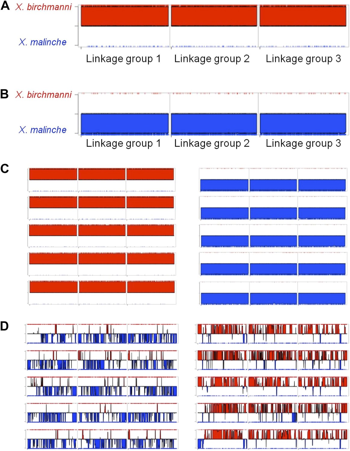
MSG ancestry plots for parental and hybrid individuals.
Representative parental individuals of X. birchmanni (A) and X. malinche (B) in linkage groups 1–3, shows that parental individuals are called as homozygous throughout the chromosome. Tick markers indicating calls to the other parent are the result of undetected polymorphism or error. More representatives from the parental panel are shown in (C). Hybrids from Tlatemaco (left) and Calnali (right) are shown in panel (D).
Figure 2 with 2 supplements

R2 distribution and p-value distributions of the sites analyzed in this study.
(A) Genome-wide distribution of randomly sampled R2 values for markers on separate chromosomes (see Figure 2—figure supplement 1 for R2 decay by distance; Figure 2—figure supplement 2 for a genome-wide plot). Blue indicates the distribution in Tlatemaco while yellow indicates the distribution in Calnali. Regions of overlapping density are indicated in green. The average genome-wide R2 in Tlatemaco is 0.003 and in Calnali is 0.006. (B) qq-plots of −log10(p-value) for a randomly selected subset of unlinked sites analyzed in this study in each population; expected p-values are drawn from p-values of the permuted data.
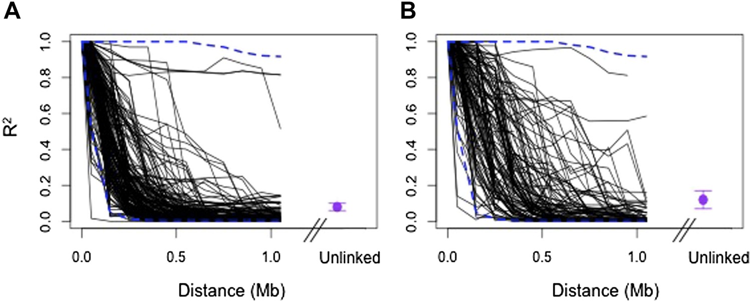
Figure 2—figure supplement 1
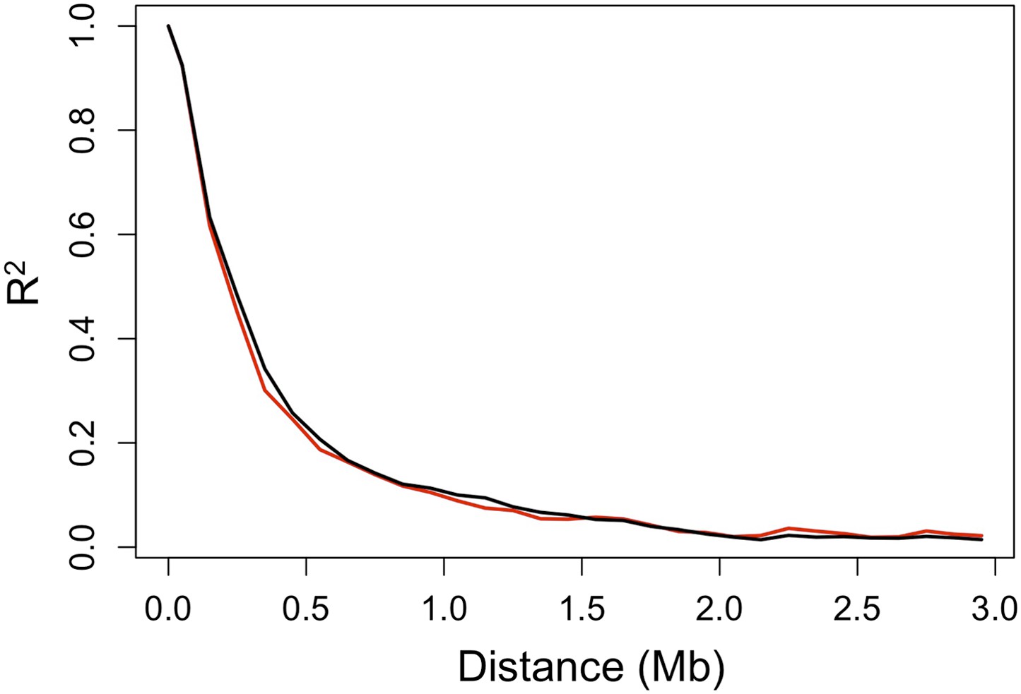
Decay in linkage disequilibrium.
Average decay of R2 over distance in Tlatemaco (black) and Calnali (red) in 100 kb windows (plot generated from 1000 randomly selected sites).
Figure 2—figure supplement 2
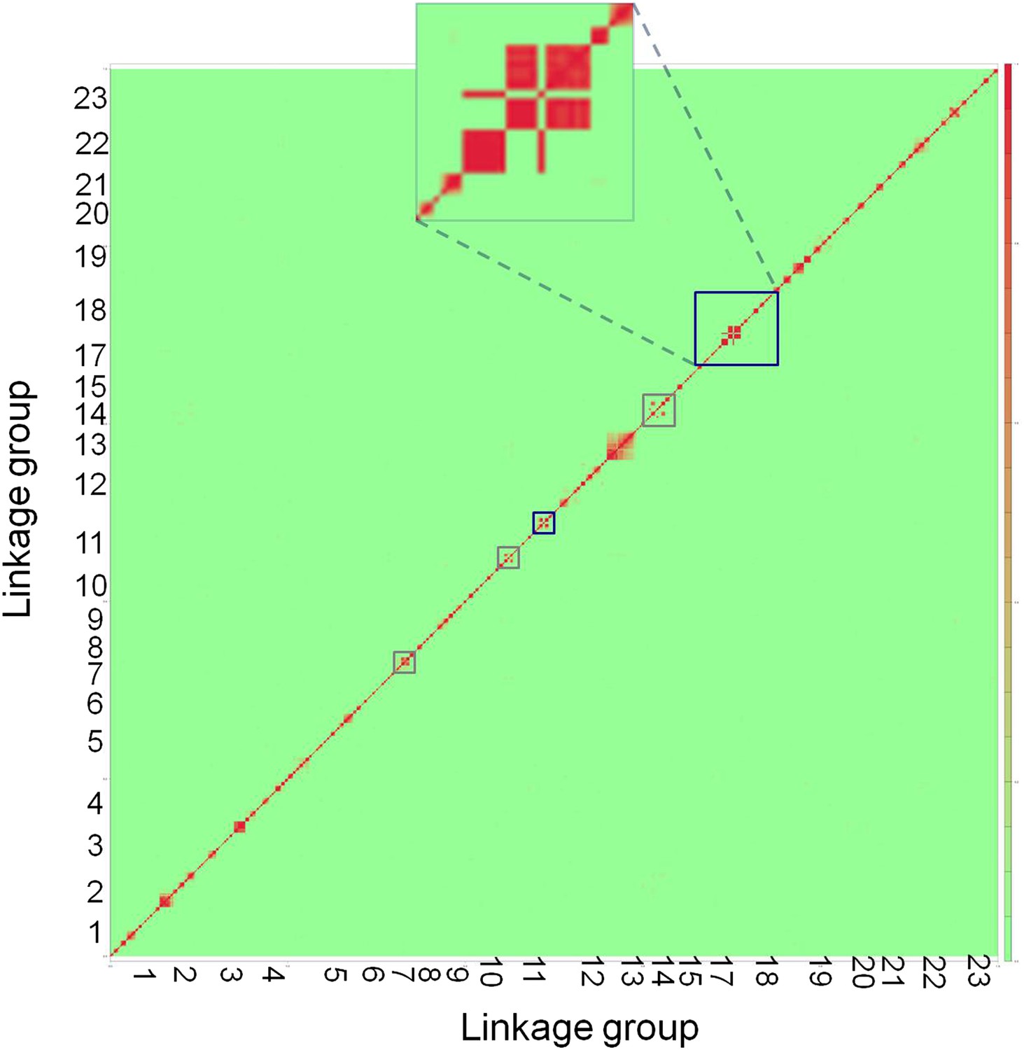
Genome-wide linkage disequilibrium plot for Tlatemaco.
This plot demonstrates that there are few regions in the X. birchmanni-malinche genomes that are inverted relative to the X. maculatus genome. Red indicates regions of R2 near 1, while green indicates low R2. Regions outlined in dark blue appear to be inverted based on the analysis in both Tlatemaco and Calnali, regions highlighted in gray appear to be inverted only in the Tlatemaco analysis.
Figure 3 with 1 supplement
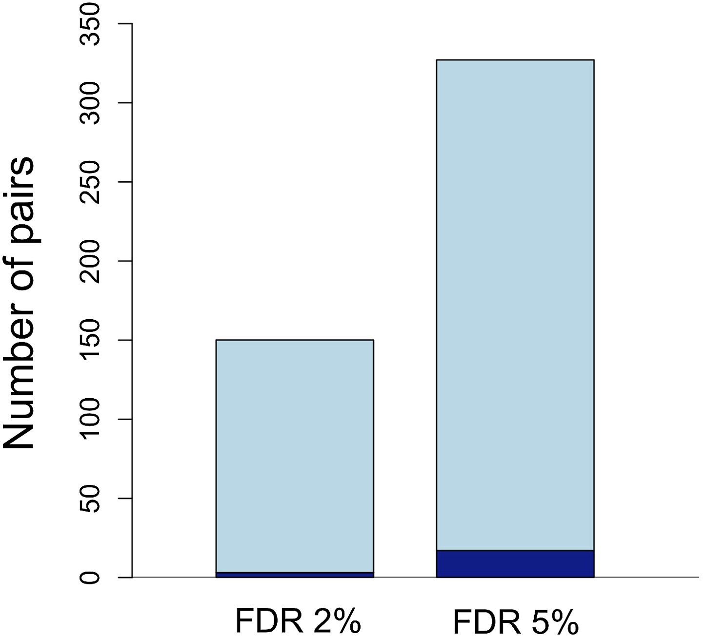
Number of unlinked pairs in significant linkage disequilibrium and expected false discovery rates.
Plot showing number of pairs of sites in significant LD in both populations in the stringent and relaxed data sets (light blue). The expected number of false positives in each data set is shown in dark blue, and was determined by simulation (see main text; Figure 3—figure supplement 1).
Figure 3—figure supplement 1
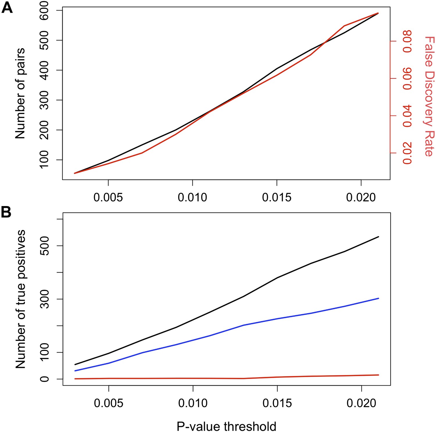
False discovery rate (FDR) at different p-value thresholds.
(A) The number of pairs of loci in LD in both populations in black (y-axis left) vs the expected false discovery rate in red (y-axis right) at different p-value thresholds. (B) Estimated number of true positives in the data set at different p-value thresholds for all pairs (black), conspecific pairs (blue), and heterospecific pairs (red). Expected false discovery rate was determined by 1000 simulations randomly permuting markers from the real data in both populations.
Figure 4 with 4 supplements

Distribution of sites in significant linkage disequilibrium throughout the Xiphophorus genome.
Schematic of regions in significant LD in both populations at FDR 5%. Regions in blue indicate regions that are positively associated in both populations (conspecific in association), regions in black indicate associations with different signs of R in the two populations, while regions in red indicate those that are negatively associated in both populations (heterospecific in association). Chromosome lengths and position of LD regions are relative to the length of the assembled sequence for that linkage group; most identified LD regions are <50 kb (Figure 4—figure supplement 1; Figure 4—figure supplement 2; Figure 4—figure supplement 3). Analysis of local LD excludes mis-assemblies as the cause of these patterns (Figure 4—figure supplement 4).
Figure 4—figure supplement 1
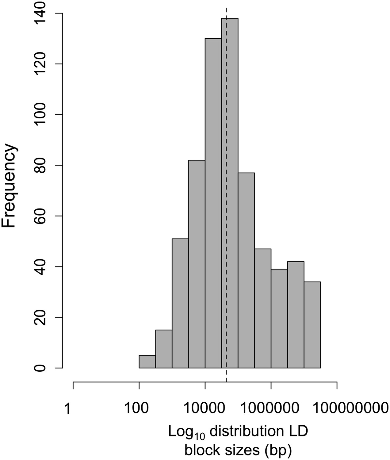
Log10 distribution of LD region length in base pairs.
The dotted line indicates the median length of regions in cross-chromosomal LD (45 kb).
Figure 4—figure supplement 2
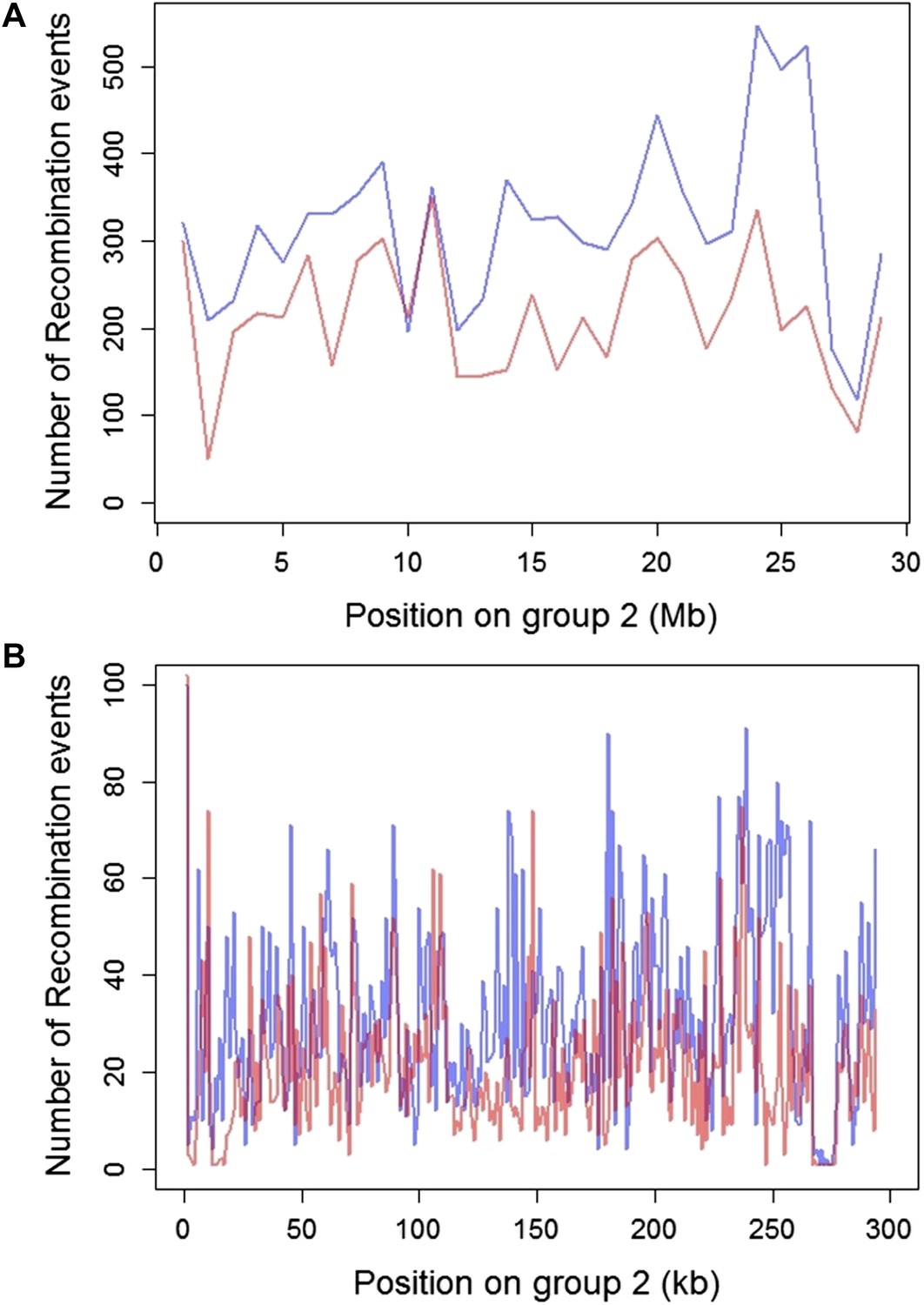
Plot of the number of recombination breakpoints detected along linkage group 2.
Number of breakpoints in Tlatemaco are indicated in blue and Calnali in red. (A) Breakpoints counted in 1 Mb windows and (B) 100 kb windows. The high density of recombination events allows for the identification of narrow regions in linkage disequilibrium.
Figure 4—figure supplement 3

Example of the use of data from two populations to narrow candidate regions in cross-chromosomal LD.
p-values for linkage disequilibrium between a marker on linkage group 2 and an interval on linkage group 16 (blue: Calnali, black: Tlatemaco). Overlapping significant intervals from the two populations allows us to narrow candidate regions.
Figure 4—figure supplement 4
Regions in cross-chromosomal LD are also in LD with their neighbors.
Decay in R2 of markers at the edge of LD blocks in both populations (black lines) compared to 95% confidence intervals of 1000 markers randomly selected from the genomic background (blue) in Tlatemaco (A) and Calnali (B). Fewer than 5% of markers fall outside of the 95% confidence intervals in each 100 kb window in both populations. Average R2 and 95% CI for regions in significant cross-chromosomal LD are shown in purple. LD blocks without neighboring markers within 300 kb of the focal marker are excluded from this figure.
Figure 5 with 3 supplements
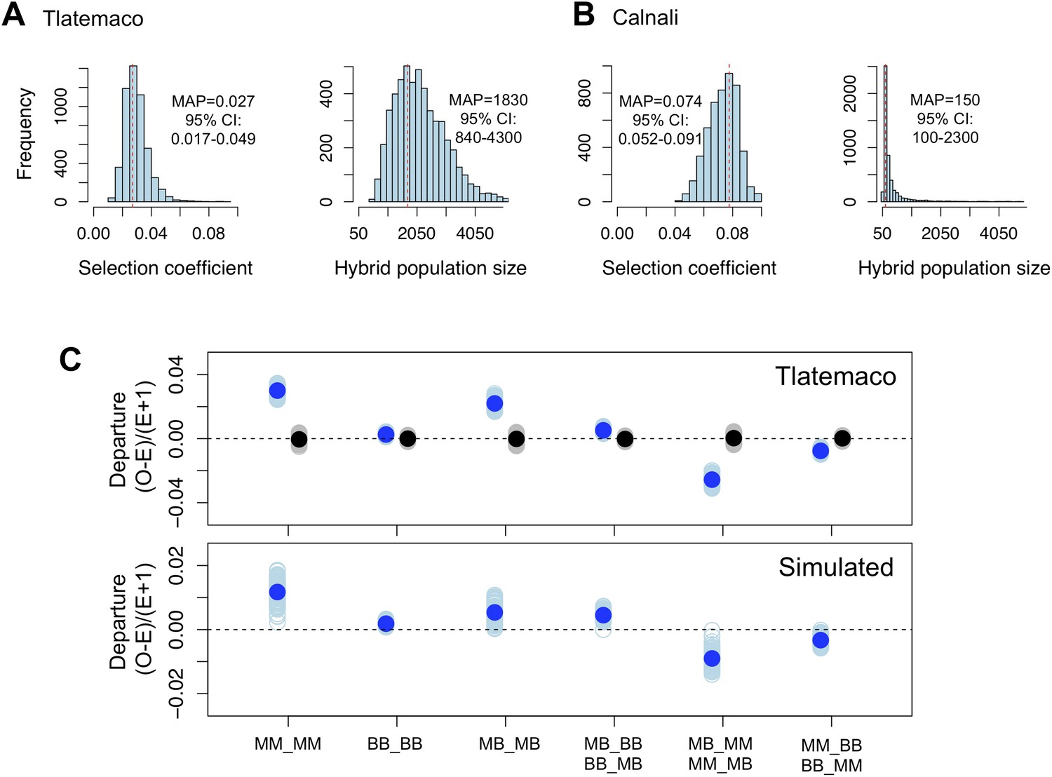
Loci in significant conspecific linkage disequilibrium show patterns consistent with selection against hybrid incompatibilities.
(A) Posterior distributions of the selection coefficient and hybrid population size from ABC simulations for Tlatemaco and (B) Calnali. The range of the x-axis indicates the range of the prior distribution, maximum a posteriori estimates (MAP) and 95% CI are indicated in the inset. (C) Departures from expectations under random mating in the actual data (top—blue points indicate LD pairs, black points indicate random pairs from the genomic background) and samples generated by posterior predictive simulations (bottom, see ‘Materials and methods’). The mean is indicated by a dark blue point; in the real data (top) smears denote the distribution of means for 1000 simulations while in the simulated data (bottom) smears indicate results of each simulation. Genotypes with the same predicted deviations on average under the BDM model have been collapsed (Figure 5—figure supplement 1, but see Figure 5—figure supplement 3) and are abbreviated in the format locus1_locus2. These simulations show that the observed deviations are expected under the BDM model. The posterior distributions for s and hybrid population size are correlated at low population sizes (Figure 5—figure supplement 2). Deviations in Calnali also follow expectations under the BDM model (Figure 5—figure supplement 3).
Figure 5—figure supplement 1

Different fitness matrices associated with selection against hybrid incompatibilities.
In a classic BDMI model (A and B), hybrid genotypes potentially under selection (indicated in red) are determined by the locus and order in which mutations occur. In a model of co-evolution between loci or extrinsic selection against hybrid phenotypes (C), more genotype combinations are potentially under selection. (A) Interaction between a mutation in locus 1 malinche and locus 2 birchmanni (two-lineage model) or first substitution occurring in locus 1 birchmanni or locus 2 malinche (one-lineage model). (B) Interaction between a mutation in locus 1 birchmanni and locus 2 malinche (two-lineage model) or first substitution occurring in locus 1 malinche or locus 2 birchmanni (one-lineage model). Format of genotypes is as follows: haplotype1_locus1-haplotype1_locus2/haplotype2_locus1-haplotype2_locus2.
Figure 5—figure supplement 2
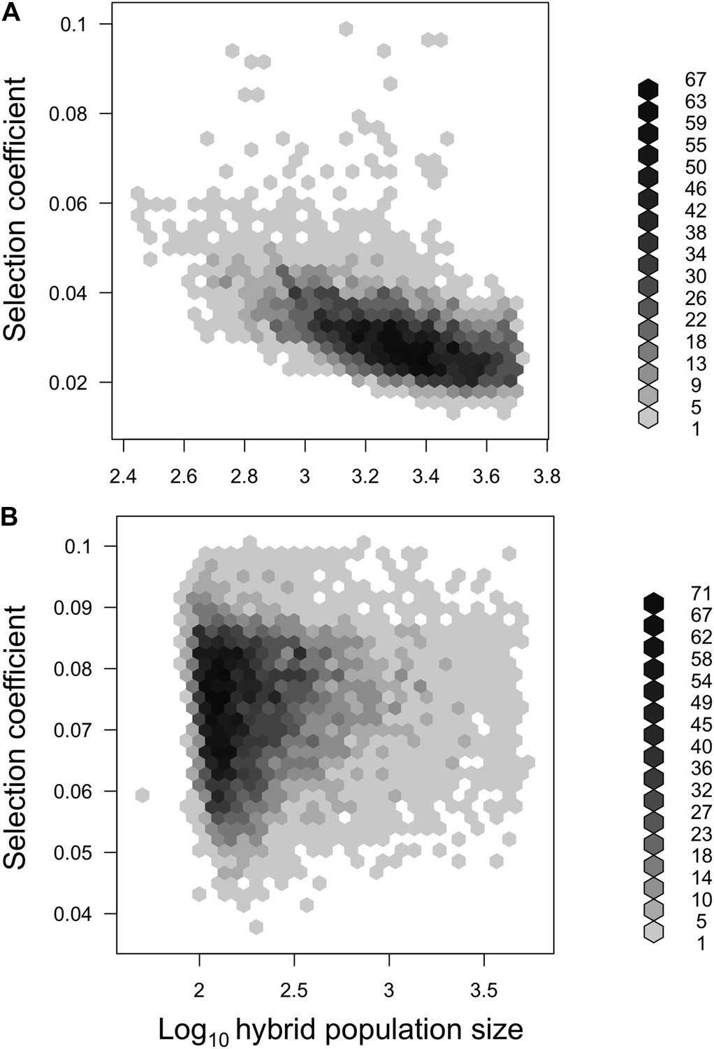
Joint posterior distribution of hybrid population size and selection coefficient.
Posterior distributions of hybrid population size and s indicate a relationship between these parameters in both populations (A-simulations of Tlatemaco, B-simulations of Calnali).
Figure 5—figure supplement 3
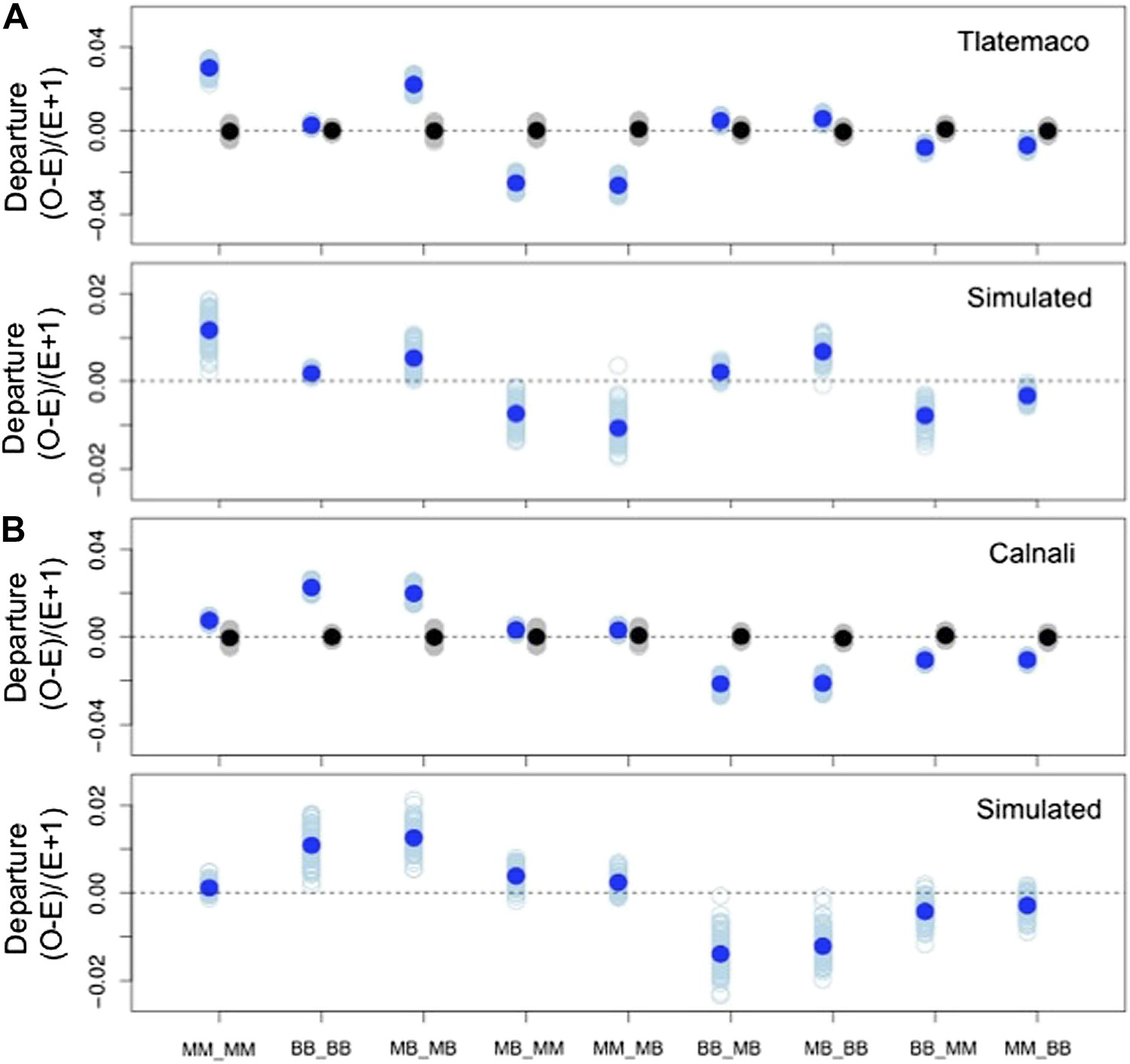
Deviations in genotype combinations compared to expected values under a two-locus selection model in both populations.
Average deviation of genotype combinations (dark blue point) from expectations under random mating at conspecific LD pairs (top) compared to posterior predictive simulations (bottom, see ‘Materials and methods’) in Tlatemaco (A) and Calnali (B). The light blue smears indicate the distribution of means for 1000 bootstrap samples in the real data and result of individual simulations in the simulated data. Labels on the x-axis indicate the genotype in the format locus1_locus2.
Figure 6
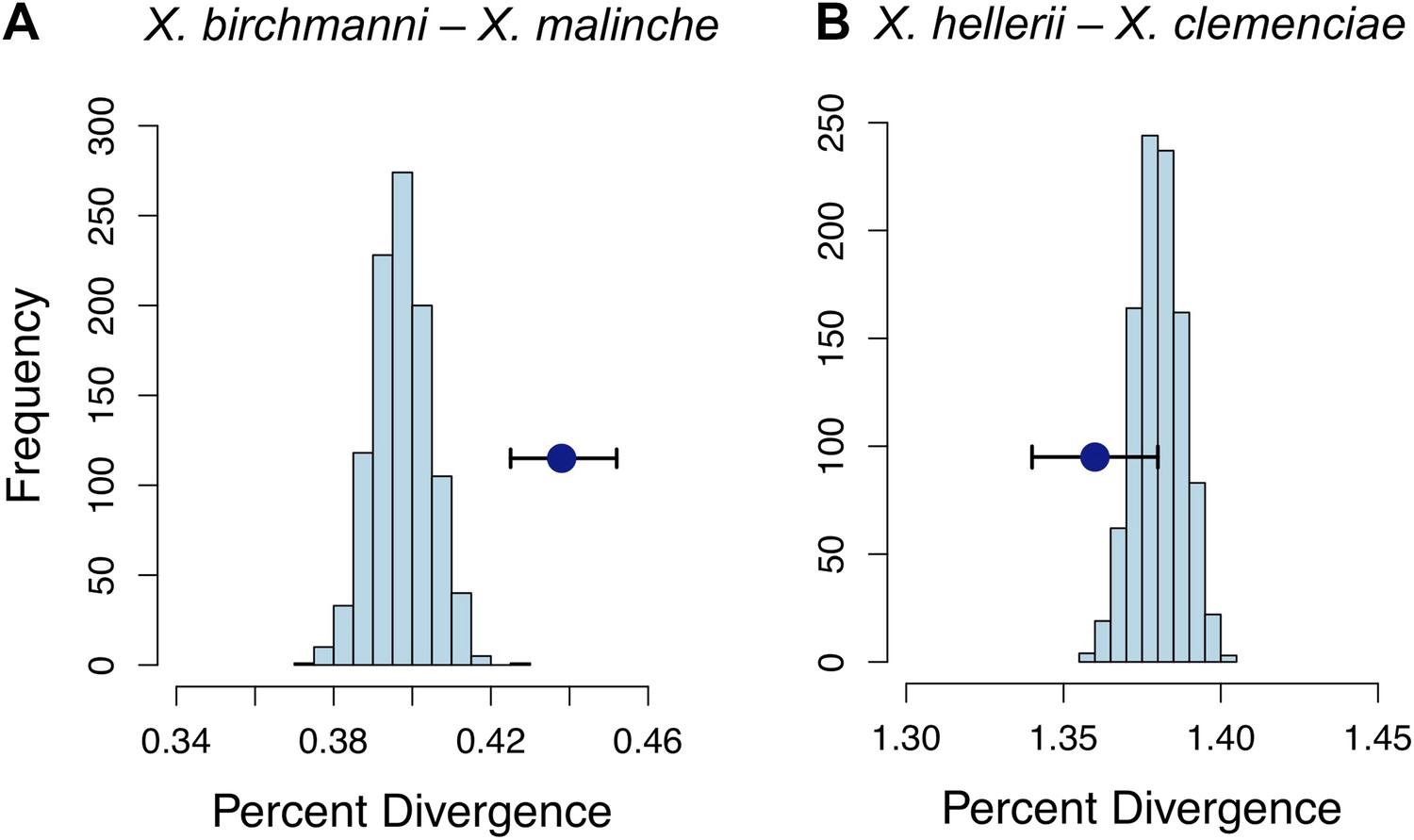
Divergence of LD pairs compared to the genomic background in two species comparisons.
(A) Regions identified in X. birchmanni and X. malinche and (B) orthologous regions in X. hellerii and X. clemenciae. The blue point shows the average divergence for genomic regions within significant LD pairs, and whiskers denote a 95% confidence interval estimated by resampling genomic regions with replacement. The histogram shows the distribution of the average divergence for 1000 null data sets generated by resampling the genomic background without replacement.
Tables
Table 1
Comparison of results for sites in significant LD at two different p-value thresholds
| Data set | Number of pairs | Proportion of pairs with conspecific associations |
|---|---|---|
| Stringent (FDR<2%) | 150 | Tlatemaco: 72% (p<0.001) Calnali: 94% (p<0.001) |
| Relaxed (FDR 5%) | 327 | Tlatemaco: 67% (p<0.001) Calnali: 94% (p<0.001) |
-
p-values were determined resampling the genomic background, see main text for details.
Table 2
Sites in significant LD are more divergent per site than the genomic background
| Mutation type | Median divergence genomic background | Median divergence stringent | Median divergence relaxed |
|---|---|---|---|
| All sites | 0.0040 | 0.0045 (p<0.001) | 0.0044 (p<0.001) |
| Nonsynonymous | 0.00040 | 0.00065 (p=0.001) | 0.00040 (p=0.6) |
| Synonymous | 0.0040 | 0.0048 (p<0.001) | 0.0045 (p=0.004) |
-
Results shown here are limited to regions that had conspecific associations in both populations (stringent dataset: 200 regions, relaxed dataset: 414 regions). p-values were determined by resampling the genomic background.
Additional files
-
Supplementary file 1
(A) Pairs of regions in significant linkage disequilibrium (FDR 5%). (B) Pairs of LD regions (FDR 5%) that have single-gene resolution. (C) Divergence analysis for full data set including pairs heterospecific in one or both populations.
- https://doi.org/10.7554/eLife.02535.022
Download links
A two-part list of links to download the article, or parts of the article, in various formats.
Downloads (link to download the article as PDF)
Open citations (links to open the citations from this article in various online reference manager services)
Cite this article (links to download the citations from this article in formats compatible with various reference manager tools)
High-resolution mapping reveals hundreds of genetic incompatibilities in hybridizing fish species
eLife 3:e02535.
https://doi.org/10.7554/eLife.02535


