Tumor evolutionary directed graphs and the history of chronic lymphocytic leukemia
- Columbia University, United States
- Amedeo Avogadro University of Eastern Piedmont, Italy
- Centro di Riferimento Oncologico, Italy
- University of Southampton, United Kingdom
- Southampton University Hospital Trust, United Kingdom
- Catholic University of the Sacred Heart, Italy
- University of Modena and Reggio Emilia, Italy
- Tor Vergata University, Italy
- Sapienza University, Italy
Figures
Figure 1 with 2 supplements
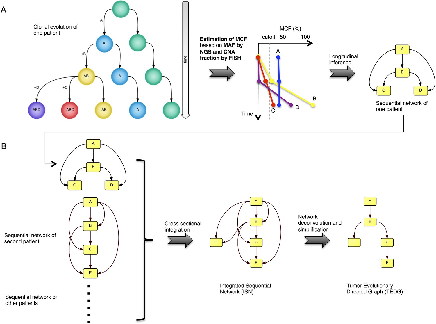
Tumor Evolutionary Directed Graph (TEDG) framework.
(A) A toy example of clonal evolution of one patient. The evolutionary history of four alterations A, B, C, and D is shown in the left panel. We then sample different time points and analyze genomic data. Specifically, for each patient, tagged-amplicon library next generation sequencing (NGS) and fluorescence in situ hybridization (FISH) analyses are carried out at different time points to evaluate the presence and quantify the clonal abundance of possible driver genetic lesions. Then we use mutation cell frequency (MCF) to adjust and unify the data (middle panel). Based on this longitudinal data, we build sequential network of one patient (right panel). CNA: copy number abnormalities. (B) Sequential networks derived from different patients (left panel) are further pooled to generate Integrated Sequential Network (ISN), which is a cross-sectional integration of longitudinal data (middle panel). We then infer TEDG by removing the indirect interactions with network deconvolution and simplification algorithms (‘Materials and methods’). To construct TEDG, we calculate a minimal spanning tree-based on the deconvolution scores (right panel).
Figure 1—figure supplement 1
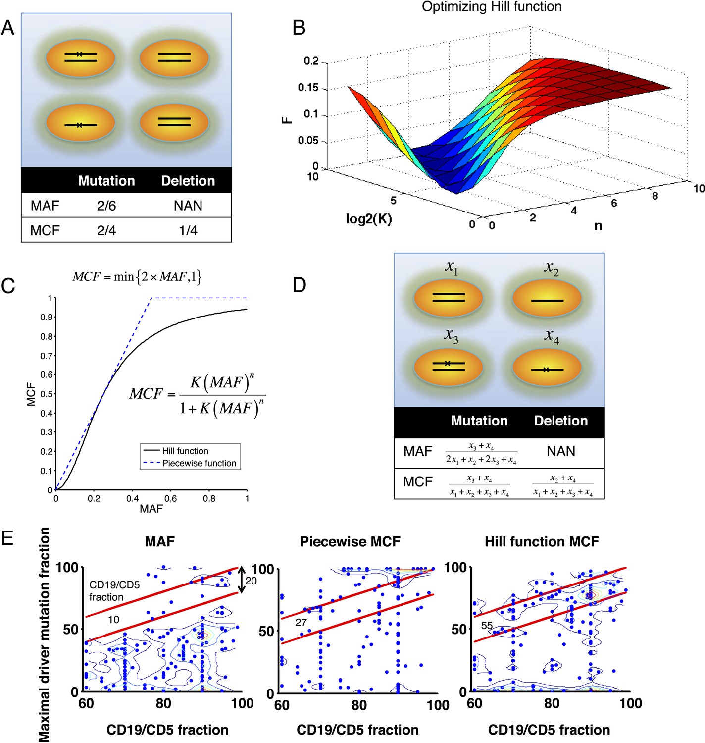
Adjustment of MAF based on copy number data.
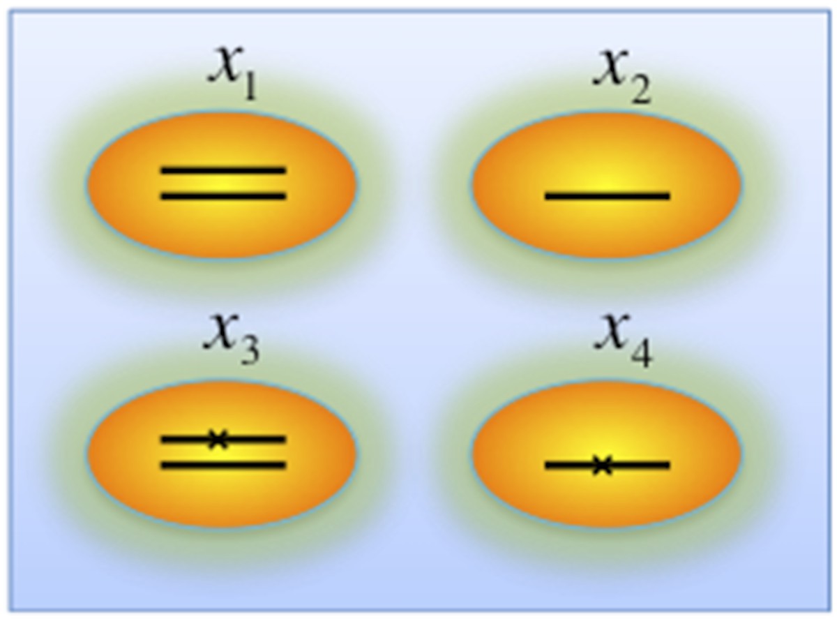
(A) Definition of mutation cell frequency. The black lines within the circles represent DNA copies, and the crosses represent point mutations. The contingent table shows the difference between MAF and MCF. MAF: mutation allele frequency; MCF: mutation cell frequency; NAN: not available. (B) Optimization of Hill function by grid-search method. z-axis indicates the objective function F, x-axis and y-axis are parameters of the Hill function. (C) The optimal Hill function and the simple piecewise function. (D) MAF and MCF of the cancer two-hit model. (E) Justification of MCF. x-axis indicates the fraction of CD19+CD5+ cells assessed by FACS analysis, and y-axis indicates the maximal mutation fraction of all targeted driver genes of each sample calculated by different methods. One blue dot represents one sample, and contours indicate the density of dots. A suitable calculation of maximal driver mutation fraction will approximate but not exceed the fraction of cancer nuclei. The upper red line indicates CD19+CD5+ cell fraction, and the lower red line indicates a 20% lower interval of it. Apparently, tumor purities of 55 samples are properly assessed by the Hill function MCF, which is better than both MAF without adjustment (10 samples) and simple piecewise MCF (27 samples).
Figure 1—figure supplement 2
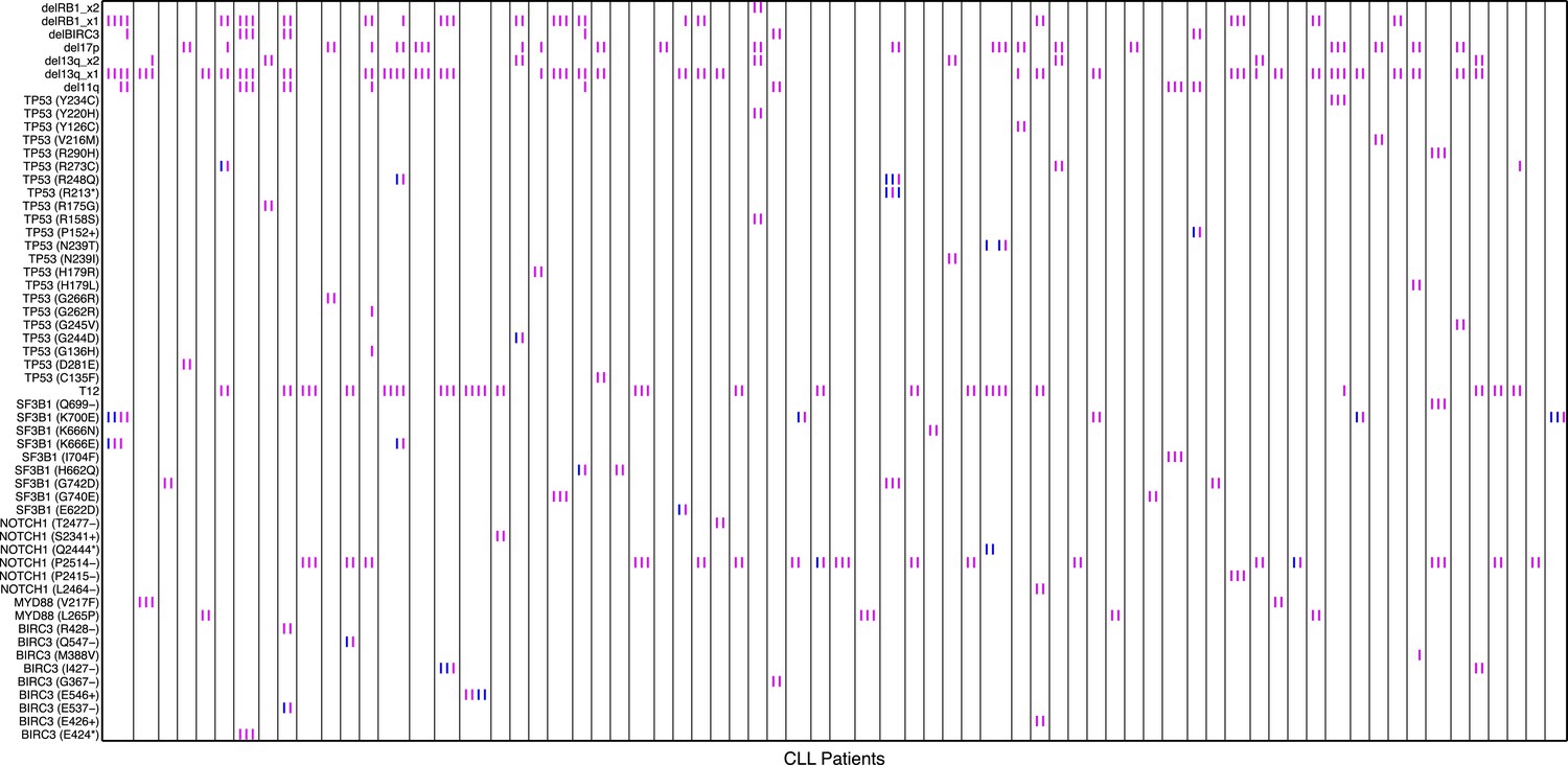
Relative timing of mutations of 70 CLL patients.
Each column represents one patient with at least two time points. Magenta (MCF > 5%, present) and blue (absent) mutations are ordered by time information, indicating the status of the corresponding alterations. For one patient, if the presence of alteration A is earlier than alteration B, we assert that A predates B.
Figure 2
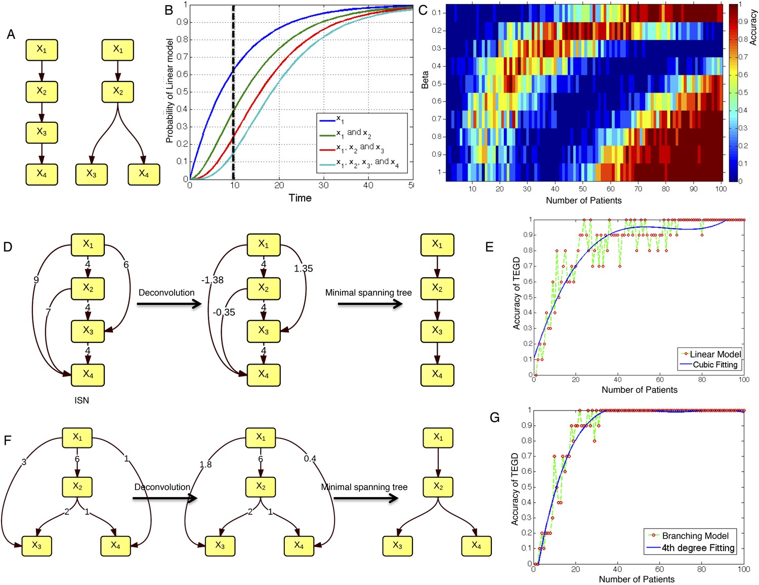
The calibration of TEDG framework on the simulation of two basic evolutionary models.
(A) The representation of linear model and branching model showing the sequential orders of four alterations. (B) The probability of observing different mutation profiles by Nordling's multi-mutation model. Specifically, if patient i harbored k0 mutations at time point t1, the probability to observe k more mutations at time point t2 is , where f represents the fitness of the new mutation. (C) The selection of parameter β. The color of heat map represents the accuracy of TEDG analysis, which is defined by the probability of TEDG reconstructing the input model. (D) An example showing the deconvolution algorithm on linear model. (F) An example showing the deconvolution algorithm on branching model. The left panel represents the ISNs of simulations of 15 patients. The weight of the edges represents the number of patients supporting the corresponding edges. The figures in the middle show the results of network deconvolution, where the numbers on the edge indicate deconvoluted weights. (E and G) The accuracy of TEDG framework on linear model and branching model at β = 0.2.
Figure 3 with 2 supplements
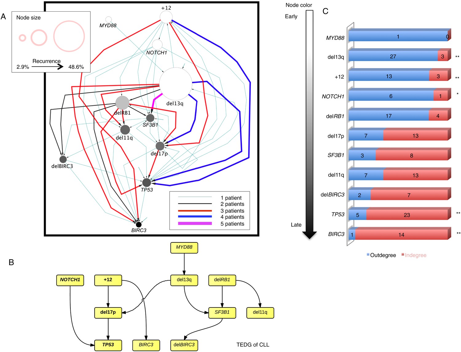
Evolutionary network analysis of CLL genetic lesions.
(A) Network representing the sequential order of genomic alterations in CLL. The nodes in the network represent genetic alterations and the oriented edges (arrows) represent sequential events in different patients where alterations in one gene predate alterations in other genes. The size of the nodes represents the recurrence of alterations in our cohort. The thickness and the color codes of the edges represent the number of patients showing a specific connection between nodes. (B) TEDG of CLL, which is the deconvolution of ISN by removing indirect interactions, representing the optimal tree to explain observed orders in CLL patients. (C) The order of CLL alterations. We calculate both the sequential in-degree (number of arrows to a node) and out-degree (number of arrows from the node) of each genetic lesion in ISN and use the binomial test to assess the significance by assuming that the number of in-degree and out-degree is randomly distributed. Our null assumption is that if there is no preferential time ordering, there should be the same number of alterations in gene A occurring before alterations in gene B and vice versa, up to statistical fluctuations. Deviations from the null assumption indicate a preferential order in the development of the alterations. All events are sorted by fold change between out-degree and in-degree and all significant early or late events are labeled by *(p-value < 0.05) or **(p-value < 0.01).
Figure 3—figure supplement 1

Summary of longitudinal data in 70 patients.
(A) The 70 patients are selected from a large cohort of 1403 CLL patients with no-bias screening. (B) The 70 patients are ranked according to their minimal cell frequency of all available genetic lesions at diagnosis. Patients with minimal cell frequency less than 20 are in red, the others are in green.
Figure 3—figure supplement 2
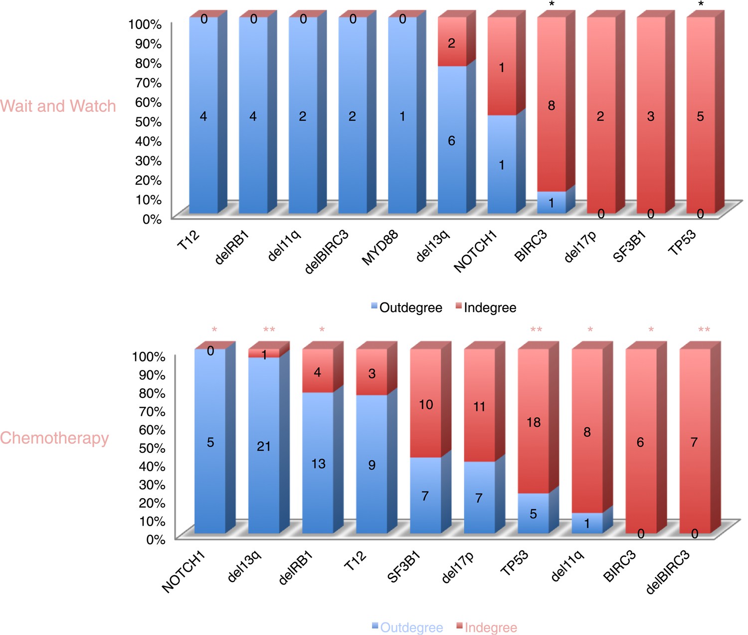
The order of CLL alterations with and without treatments.
All events are sorted by fold change between in-degree and out-degree, and all significant early or late events are labeled by *(p-value < 0.05) or **(p-value < 0.01). The upper panel represents the results of patients with only watch and wait, while the lower panel represents the results of patients with treatment.
Figure 4 with 1 supplement
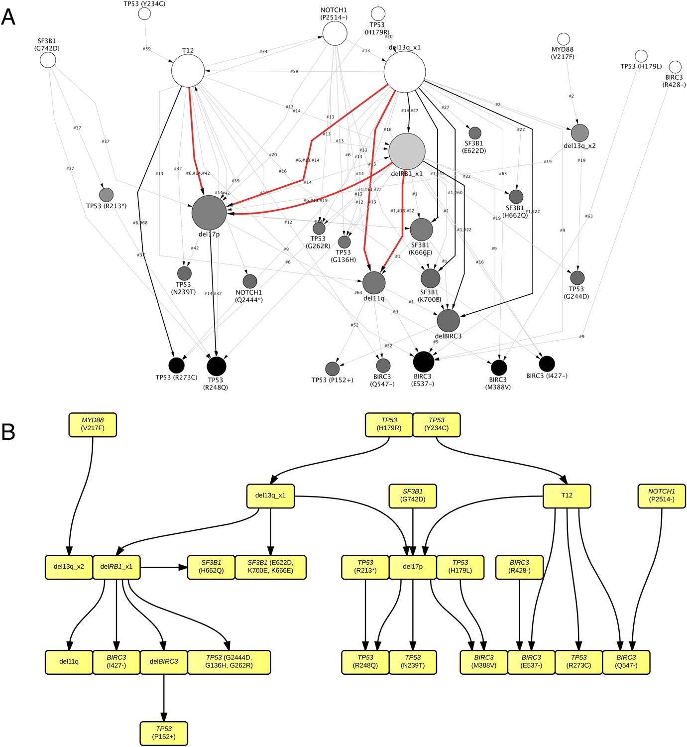
TEDG analysis of specific genetic lesions.
(A) Network representing the sequential order of specific genomic alterations. Two alterations are connected by a directed edge if they are observed to successively appear in at least one patient. The patient ID labels the corresponding edges, which are further colored by the number of patients. Nodes are colored by the fold change between out-degree and in-degree, indicating temporal order of corresponding alterations. The size of the nodes represents the recurrence of the alteration. (B) Tumor Evolutionary Directed Graph of 32 specific mutations. Some nodes and arrows in this figure are manually merged or adjusted for the purpose of illustration.
Figure 4—figure supplement 1
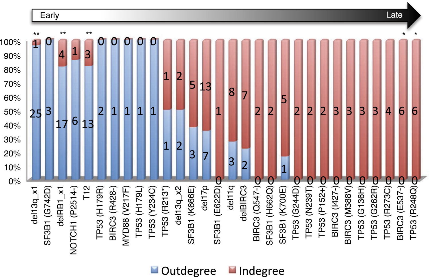
Statistical test of in-degree and out-degree of specific alterations.
All alterations are ranked by fold change between in-degree and out-degree.
Figure 5
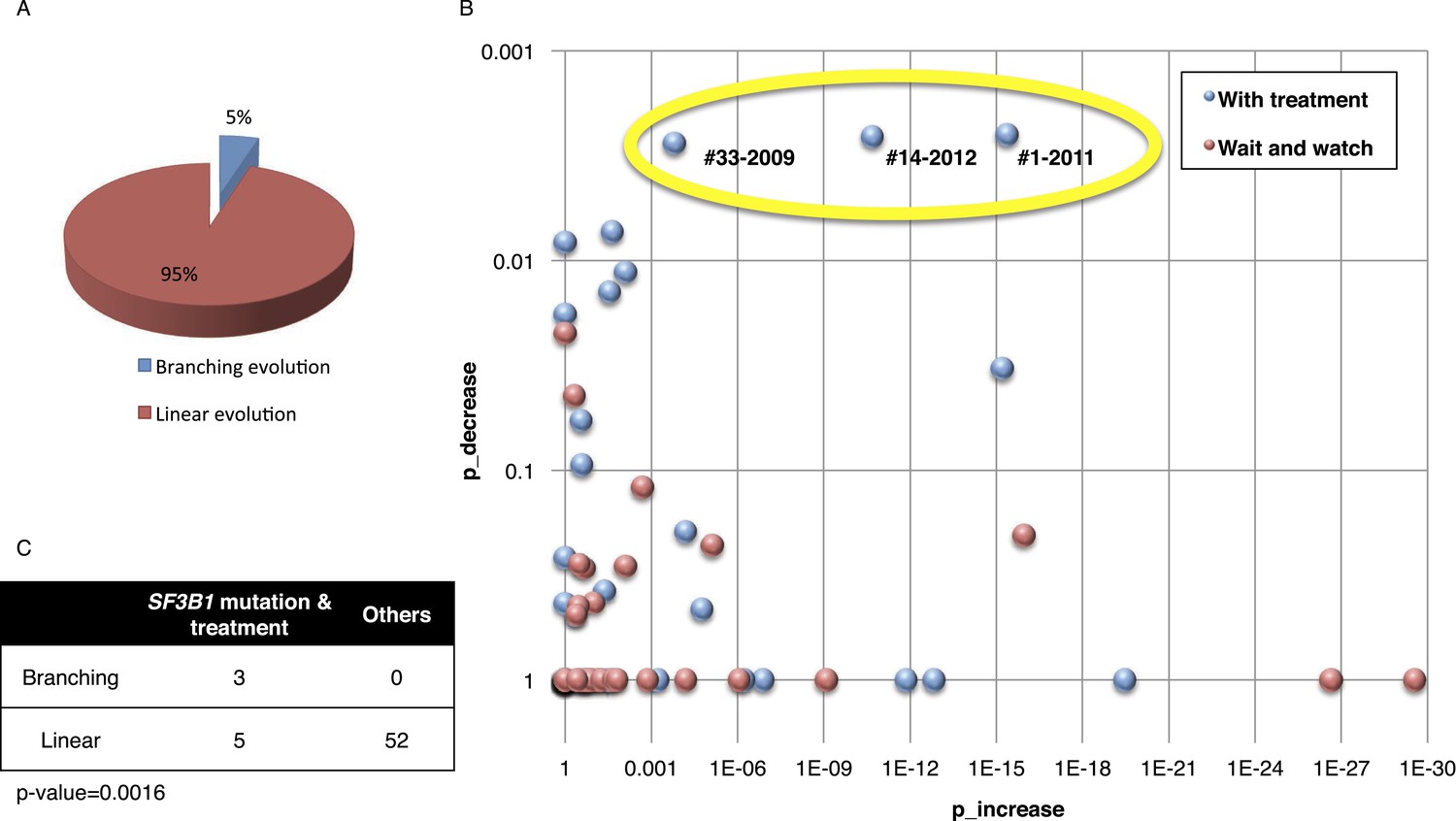
Fitting the evolution models.
(A) Distribution of the clonal evolution pattern in the 60 non-Richter cases. Three of the 60 cases show replacement during tumor progression. (B) Scatter plot showing p-values of observing increased and decreased subclones in the 80 samples of the 60 multi-time point patients. Samples with evidence of clonal replacement are located in the right-up corner (highlighted by yellow circle). (C) Number of patients following linear vs branched evolution pattern according to SF3B1 mutational emergence and previous treatment (p-value 0.0016 by Fisher's exact test).
Figure 6 with 3 supplements

Association network of CLL lesions in a larger cohort.
(A) The mutation status of 1054 CLL patients, which is informative in 11 most common genetic lesions in this leukemia. (B) The association analysis of CLL genetic lesions in TEDG. Lesion pairs are connected if they are significantly co-mutated (red) or mutually exclusive (blue). (C) Box plot of growth rate of all genetic lesions.
Figure 6—figure supplement 1

Box plot to show the difference of Richter and non-Richter, and mutations of TP53 in Maximal Mutation Frequency Slope.
https://doi.org/10.7554/eLife.02869.015
Figure 6—figure supplement 2
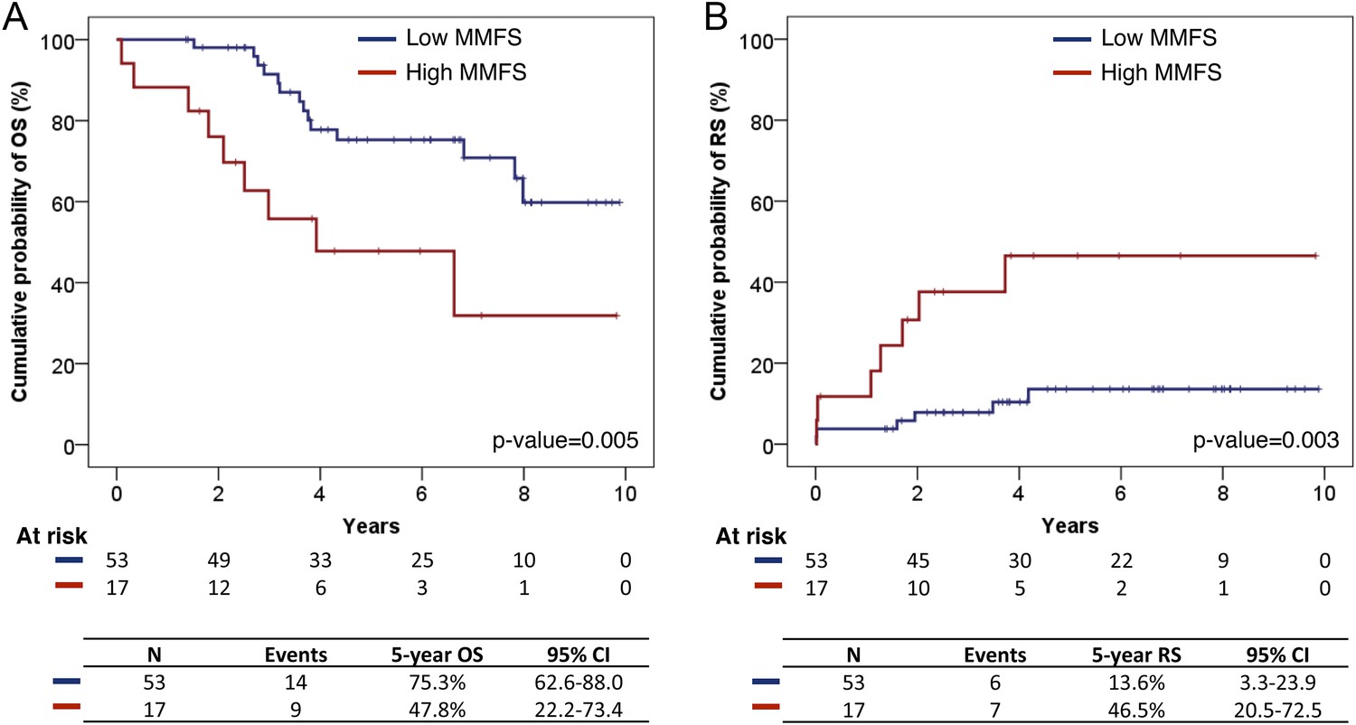
Survival analysis of fittest genomic alterations.
(A) Kaplan–Meier curve showing the cumulative probability of overall survival (OS) for patients with high and low MMFS (maximal mutation frequency slope). (B) Kaplan–Meier curve showing the cumulative probability of Richter syndrome (RS) transformation for patients with high and low MMFS. p-values are based on log-rank test. CI (confidential interval) is estimated by the Greenwood method.
Figure 6—figure supplement 3
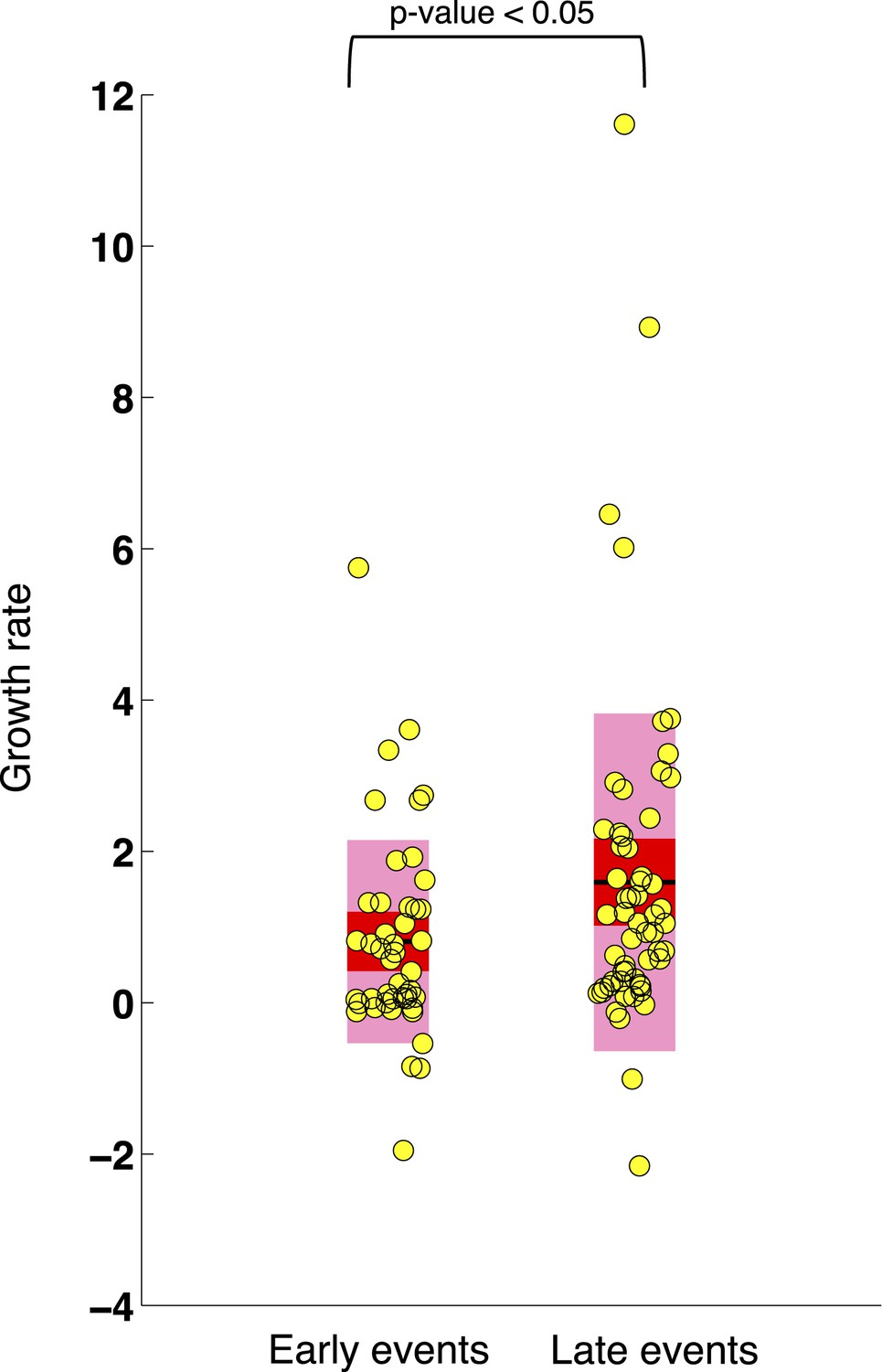
Comparison of the growth rates of subclonal alterations between early and late events.
p-value is calculated by Wilcoxon Rank-Sum Test. Growth rate indicates the change of mutation frequency per year.
Author response image 1
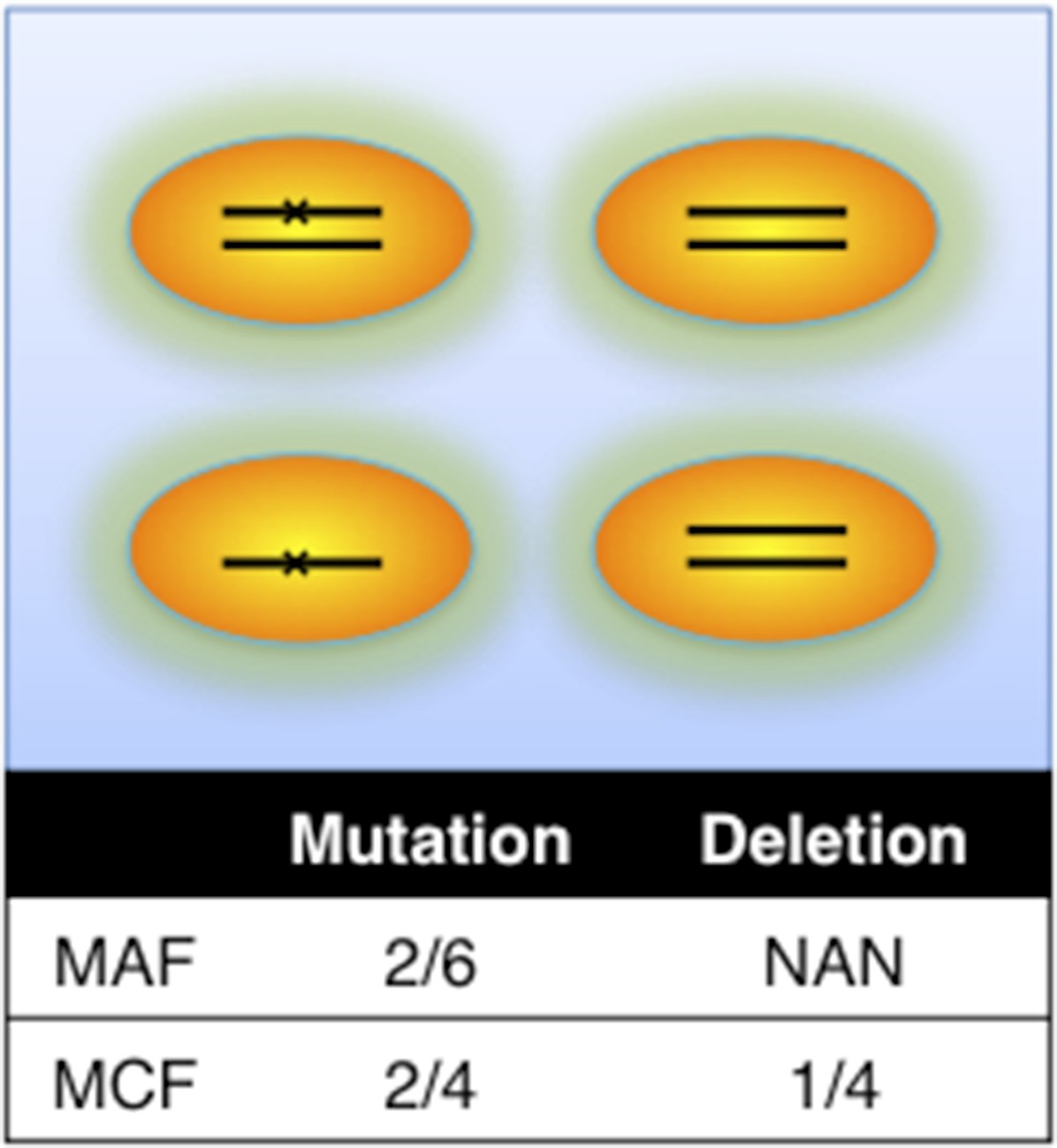
Definition of mutation cell frequency.
MAF: mutation allele frequency; MCF: mutation cell frequency. The black lines within the circles represent DNA copies, and the crosses represent mutations. The contingent table shows the difference between MAF and MCF.
Author response image 2
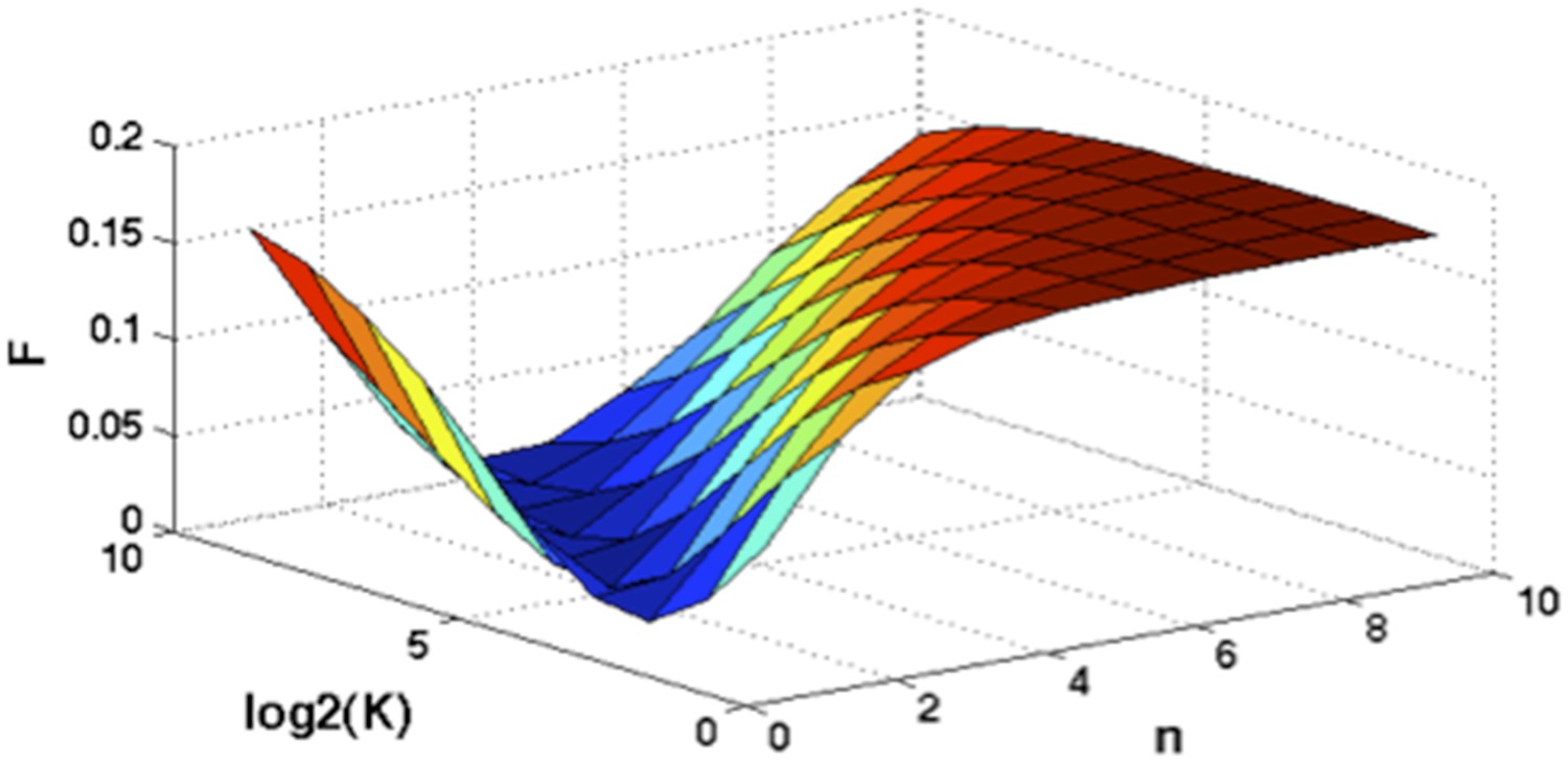
Optimization of Hill function by grid search method.
z-axis indicates the objective function, x-axis and y-axis are parameters of Hill function.
Author response image 3

Optimal correlation between MAF and MCF.
Author response image 4
Genotypes of two-hit model.
Black lines within the circles represent copies of DNA, and crosses on the lines indicates point mutations. χ1, χ2, χ3, and χ4 indicate proportion of the cells with corresponding genotype.
Author response image 5
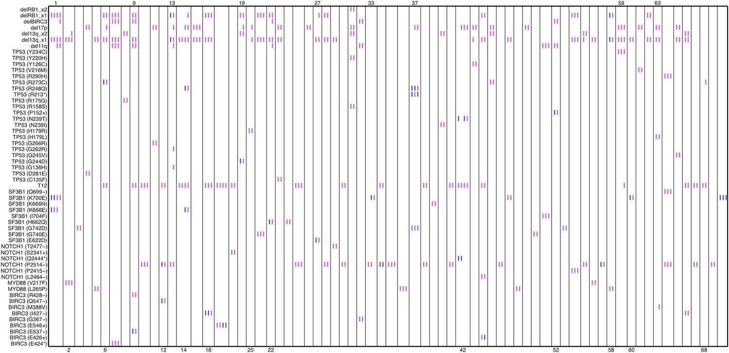
Relative timing of mutations of 70 patients.
Each column represents one patient with at least two time points. Magenta (MCF>5%, present) and blue bars (absent), which are ordered by time information, indicate the mutation status of the corresponding alteration. For one patient, if the present of alteration A is earlier than B, we claim A predates B.
Author response image 6
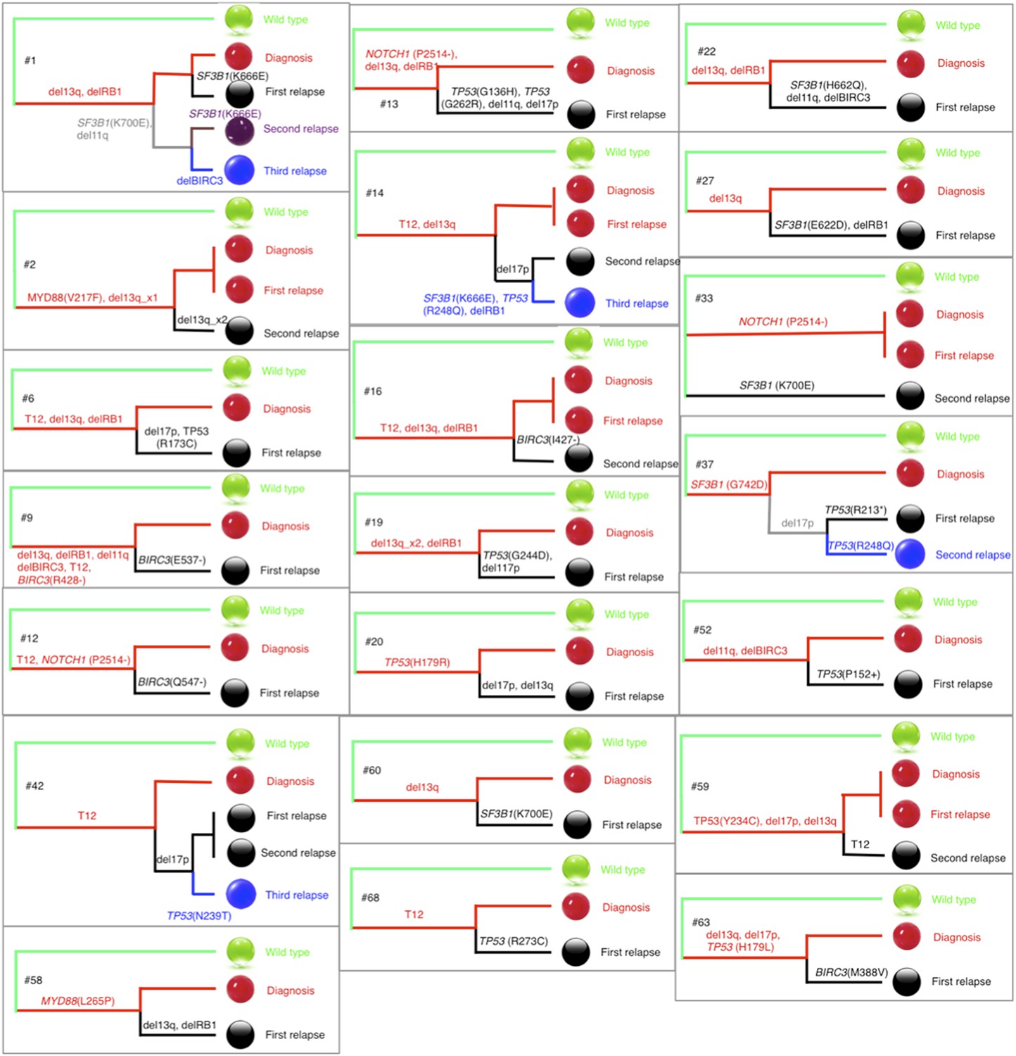
Phylogenetic trees of CLL patients.
Twenty-one out of all CLL patients contain the change of mutation status during disease progression. The phylogenetic trees are constructed based on mutation status of the driver genes. Green balls are normal cells, while all the others are cancer cells with particular alterations.
Author response image 7
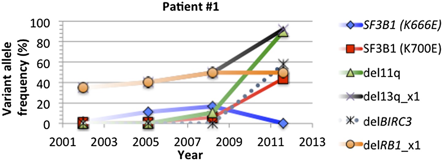
Change of mutation frequency of patient #1.
There are four samples for patient #1. Mutation frequencies of different alterations change according to the progression of the disease.
Author response image 8
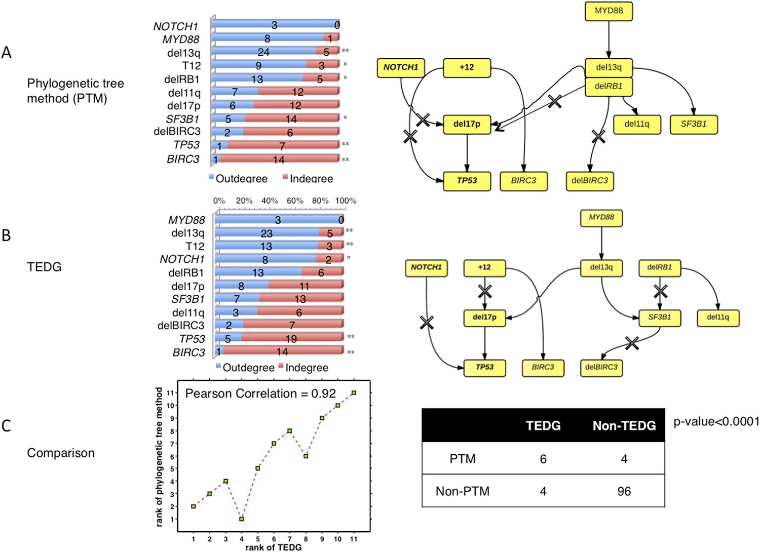
The comparison between TEDG (B) and phylogenetic tree method (A).
The two methods are compared in terms of the order of mutations and the TEDG networks. * indicates p-value<0.05, and ** indicates p-value<0.01. p-value in (C) is calculated by Fisher’s exact test.
Author response image 9
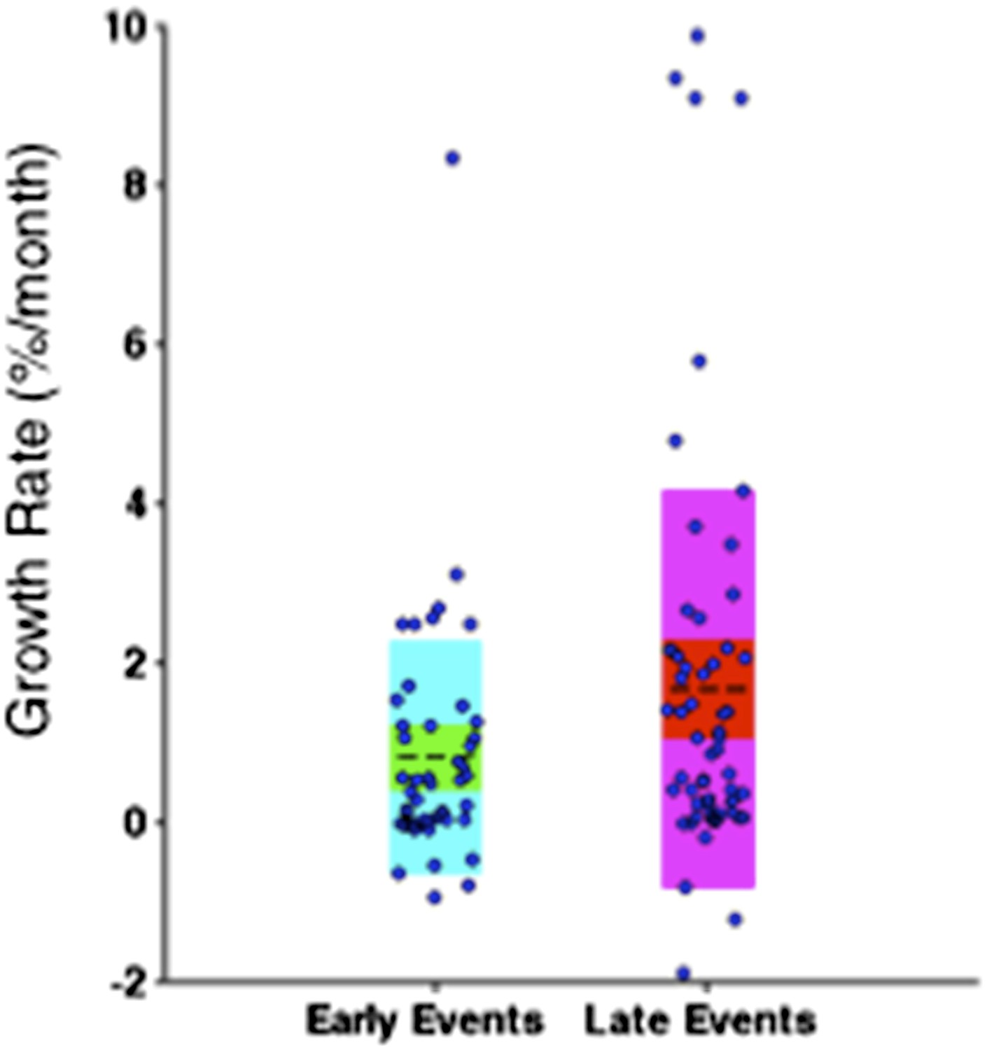
Comparison of the growth rate of subclonal alterations between early and late events.
Author response image 10

Summary of longitudinal data in 70 patients.
(A) The 70 patients are selected from a big cohort of 1,403 CLL patients with no-bias screening. (B) 70 patients are ranked according to their minimal cell frequency at diagnosis. Patient with minimal cell frequency less than 20 are in red, the others are in green.
Author response image 11

The impact of sampling error on MCF.
Confidence interval of MCF is inferred based on the variation of MAF estimated by dilution experiments.
Author response image 12
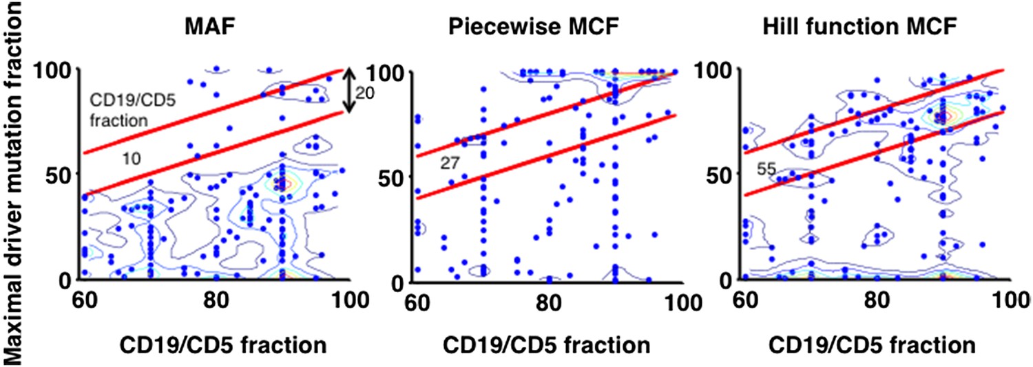
Justification of MCF.
X-axis indicates fraction of CD19+CD5+ cells assessed by FACS analysis, and y-axis indicates maximal mutation fraction of all targeted driver genes of each sample calculated by different methods. One blue dot represents one sample, and contours indicate the density of dots. A suitable calculation of maximal driver mutation fraction will approximate but not exceed the fraction of cancer nuclei. The upper red line indicates CD19+CD5+ cell fraction, and the lower red line indicates a 20% lower interval of it. Apparently, tumor purities of 55 samples are properly assessed by the Hill function MCF, which is better than both MAF without adjustment (10 samples) and simple piecewise MCF (27 samples).
Author response image 13
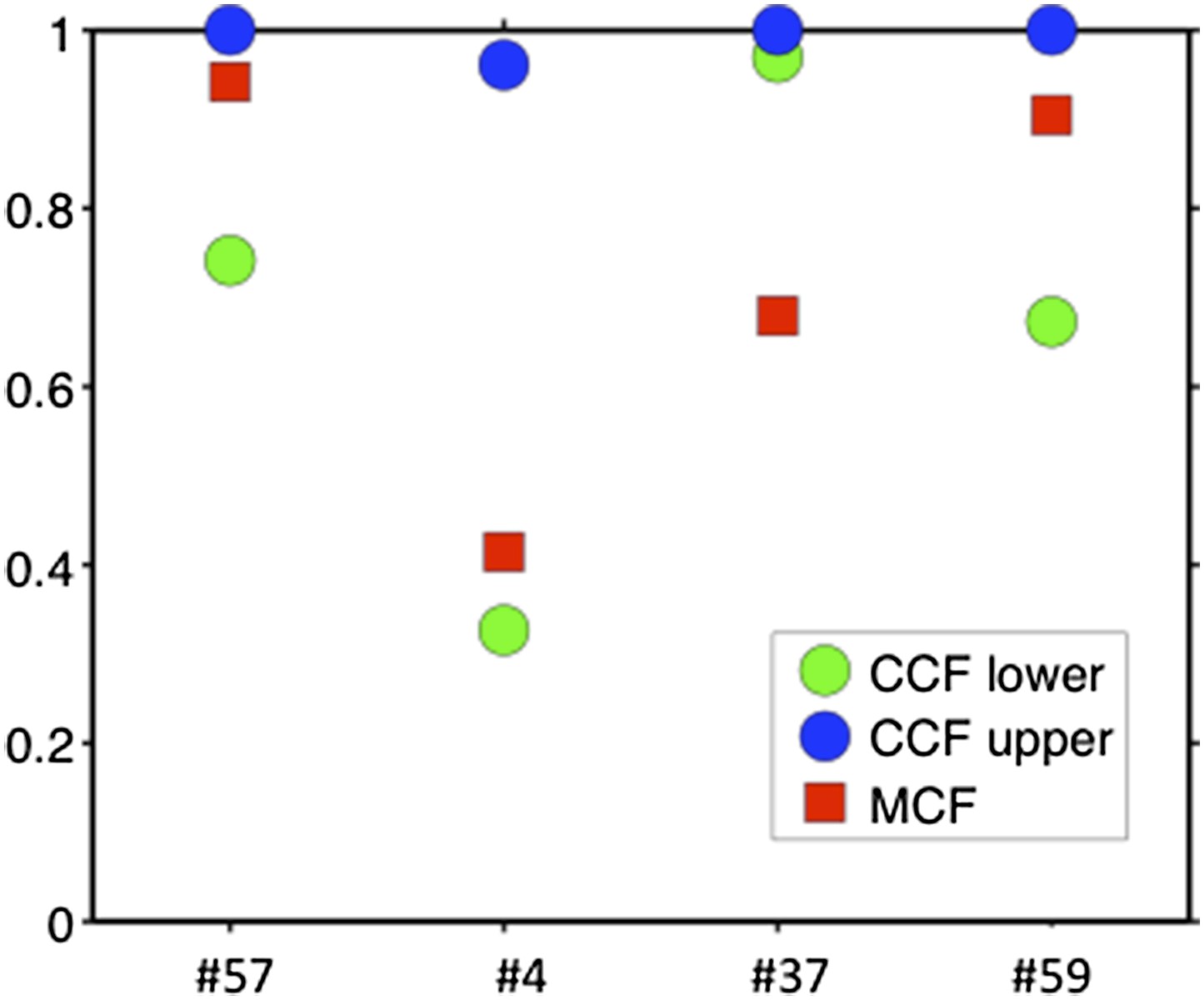
Comparison of MCF and CCF.
The samples with WES available show that our MCF falls within the estimates of ABSOLUTE. ABSOLUTE underestimates tumor purity in sample #37 as compared to CD19/CD5 FACS and our MCF estimate.
Author response image 14
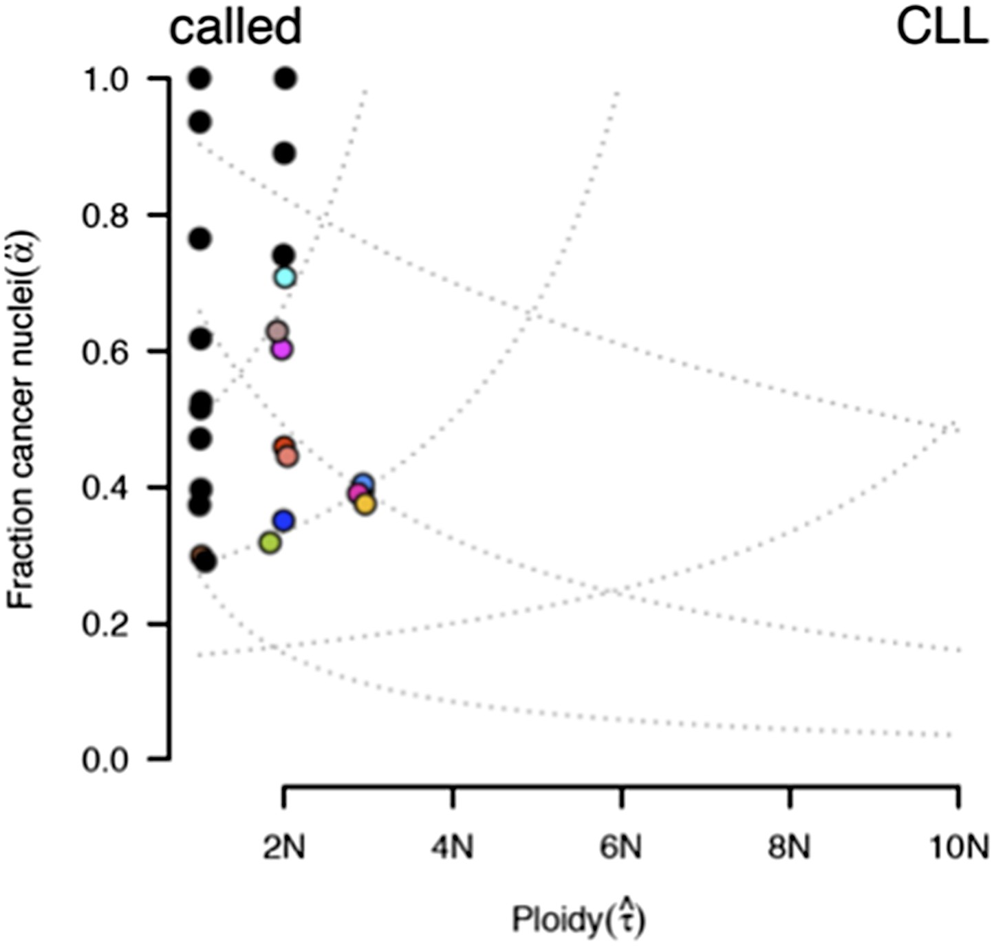
ABSOLUTE report of case #37.
Several models fit the data with different purity estimates.
Tables
Table 1
Patients with branching evolution*
| Patient ID | Sampling time | Treatment | Increased alterations | Decreased alterations | Detectable alterations |
|---|---|---|---|---|---|
| #1 | 2001 | None | – | – | SF3B1 (K666E), SF3B1 (K700E), del13q |
| 2005 | FC | SF3B1 (K666E) | None | SF3B1 (K666E), SF3B1 (K700E), del13q | |
| 2008 | FCR/CAM/RBEN | SF3B1 (K700E), del11q | None | SF3B1 (K666E), SF3B1 (K700E), del13q, del11q | |
| 2011 | BENCAM | SF3B1 (K700E), del11q, del13q, delBIRC3 | SF3B1 (K666E) | SF3B1 (K700E), del13q, del11q, delBIRC3 | |
| #14 | 2004 | RF | – | – | +12, del13q |
| 2007 | FC/CAM | None | None | +12, del13q | |
| 2010 | BENCAM | TP53 (R248Q), del17p, SF3B1 (K666E) | None | +12, del13q, TP53 (R248Q), del17p, SF3B1 (K666E) | |
| 2012 | BENDOFA | TP53 (R248Q), del17p, SF3B1 (K666E), T12 | del13q | +12, del13q, TP53 (R248Q), del17p, SF3B1 (K666E) | |
| #33 | 2002 | None | – | – | NOTCH1 (P2514-) |
| 2004 | FCR | SF3B1 (K700E) | None | NOTCH1 (P2514-), SF3B1 (K700E) | |
| 2009 | FCR | SF3B1 (K700E) | NOTCH1 (P2514-) | SF3B1 (K700E) |
-
*
FC, fludarabine, cyclophosphamide; FCR, fludarabine, cyclophosphamide, rituximab; CAM, Campath; RBEN, rituximab, bendamustine; BENCAM, bendamustine, Campath; RF, rituximab, fludarabine; BENDOFA, bendamustine, ofatumumab.
Table 2
Clinical features at presentation of the CLL cohorts*
| TEDG analysis | SA analysis | |||||
|---|---|---|---|---|---|---|
| N | Total | % | N | Total | % | |
| IGHV homology >98% | 37 | 69 | 53.6 | 532 | 1380 | 38.6 |
| del13q14 | 35 | 70 | 50.0 | 682 | 1403 | 48.6 |
| +12 | 19 | 70 | 27.1 | 205 | 1403 | 14.6 |
| del11q22-q23 | 8 | 70 | 11.4 | 136 | 1403 | 9.7 |
| del17p13 | 20 | 70 | 28.6 | 114 | 1403 | 8.1 |
| TP53 mutation | 22 | 70 | 31.4 | 114 | 1401 | 8.1 |
| NOTCH1 mutation | 22 | 70 | 31.4 | 150 | 1403 | 10.7 |
| SF3B1 mutation | 17 | 70 | 24.3 | 100 | 1403 | 7.1 |
| MYD88 mutation | 6 | 70 | 8.6 | 52 | 1403 | 3.7 |
| BIRC3 mutation | 10 | 70 | 14.3 | 41 | 1403 | 2.9 |
| BIRC3 deletion | 6 | 70 | 8.6 | 79 | 1403 | 5.6 |
-
*
TEDG analysis, Tumor Evolutionary Directed Graphs analysis; SA analysis, Statistical Association analysis; IGHV, immunoglobulin heavy variable gene; FISH, fluorescence in situ hybridization.
Table 3
Patients showing high maximal mutation frequency slope (MMFS)
| Patient | MMFS* | Fast growing mutations | MCF1 (%) | MCF2 (%) | dT (moths) | Treatment | Richter syndrome transformation |
|---|---|---|---|---|---|---|---|
| #52 | 117.7 | TP53 (P152+) | 2.1 | 11.4 | <1 | None | Yes |
| #68 | 9.1 | TP53 (R273C) | 0.0 | 100.0 | 11 | None | No |
| #51 | 6.7 | SF3B1 (I704F) | 12.2 | 68.9 | 5 | RCVP | Yes |
| #37 | 6.4 | TP53 (R248Q) | 3.8 | 90.0 | 10 | RDHAOX | Yes |
| #57 | 5.9 | NOTCH1 (P2514-) | 0.8 | 94.2 | 12 | None | Yes |
| #47 | 4.6 | del13q | 37.6 | 100.0 | 13 | None | No |
| #14 | 3.9 | del17p | 18.9 | 90.0 | 16 | A | No |
| #42 | 3.4 | TP53 (N239T) | 0.0 | 100.0 | 16 | RDHAOX | Yes |
| #4 | 3.3 | del17p | 53.6 | 100.0 | 15 | CLB-O | No |
| #54 | 3.0 | NOTCH1 (P2415-) | 100.0† | 100.0 | 22 | FCO | No |
| #22 | 2.9 | BIRC3 deletion | 0.0 | 93.9 | 29 | FCR | No |
| #20 | 2.8 | del13q | 0.0 | 100.0 | 36 | CLB | No |
| #63 | 2.5 | BIRC3 (M388V) | 0.0 | 86.0 | 24 | FCR | Yes |
| #6 | 2.3 | del17p | 0.0 | 92.1 | 34 | CLB | No |
| #38 | 2.3 | NOTCH1 (P2514-) | 41.7 | 42.9 | 4 | CVP | Yes |
| #13 | 2.2 | TP53 (G136H) | 0.0 | 100.0 | 45 | RDHAOX | No |
| #1 | 2.1 | del11q | 11.8 | 100.0 | 41 | FCR/A/BR | No |
-
*
MMFS, maximal mutation frequency slope (in standard deviation per year); MCF1, mutation cell frequency of selected mutation at the first time point; MCF2, mutation cell frequency at the second time point; dT, the elapsed time between two samples; RCVP, rituximab, cyclophosphamide, vincristine, prednisone; RDHAOX, rituximab, dexamethasone, high dose cytarabine, oxaliplatin; A, alemtuzumab; CLB-O, chlorambucil, ofatumumab; FCO, fludarabine, cyclophosphamide, ofatumumab; FCR, fludarabine, cyclophosphamide, rituximab; CLB, chlorambucil; CVP, rituximab, cyclophosphamide, vincristine, prednisone; BR, bendamustine, rituximab.
-
†
Total number of the cancer cells with NOTCH1 alteration does not change, but the allele frequency of the mutation increases because of the deletion of the wild-type allele.
Additional files
-
Supplementary file 1
PCR primers and conditions.
- https://doi.org/10.7554/eLife.02869.020
-
Supplementary file 2
FACS Data.
- https://doi.org/10.7554/eLife.02869.021
Download links
A two-part list of links to download the article, or parts of the article, in various formats.
Downloads (link to download the article as PDF)
Open citations (links to open the citations from this article in various online reference manager services)
Cite this article (links to download the citations from this article in formats compatible with various reference manager tools)
Tumor evolutionary directed graphs and the history of chronic lymphocytic leukemia
eLife 3:e02869.
https://doi.org/10.7554/eLife.02869


