Human premotor areas parse sequences into their spatial and temporal features
- University College London, United Kingdom
- Erasmus Medical Centre, Netherlands
Figures
Figure 1
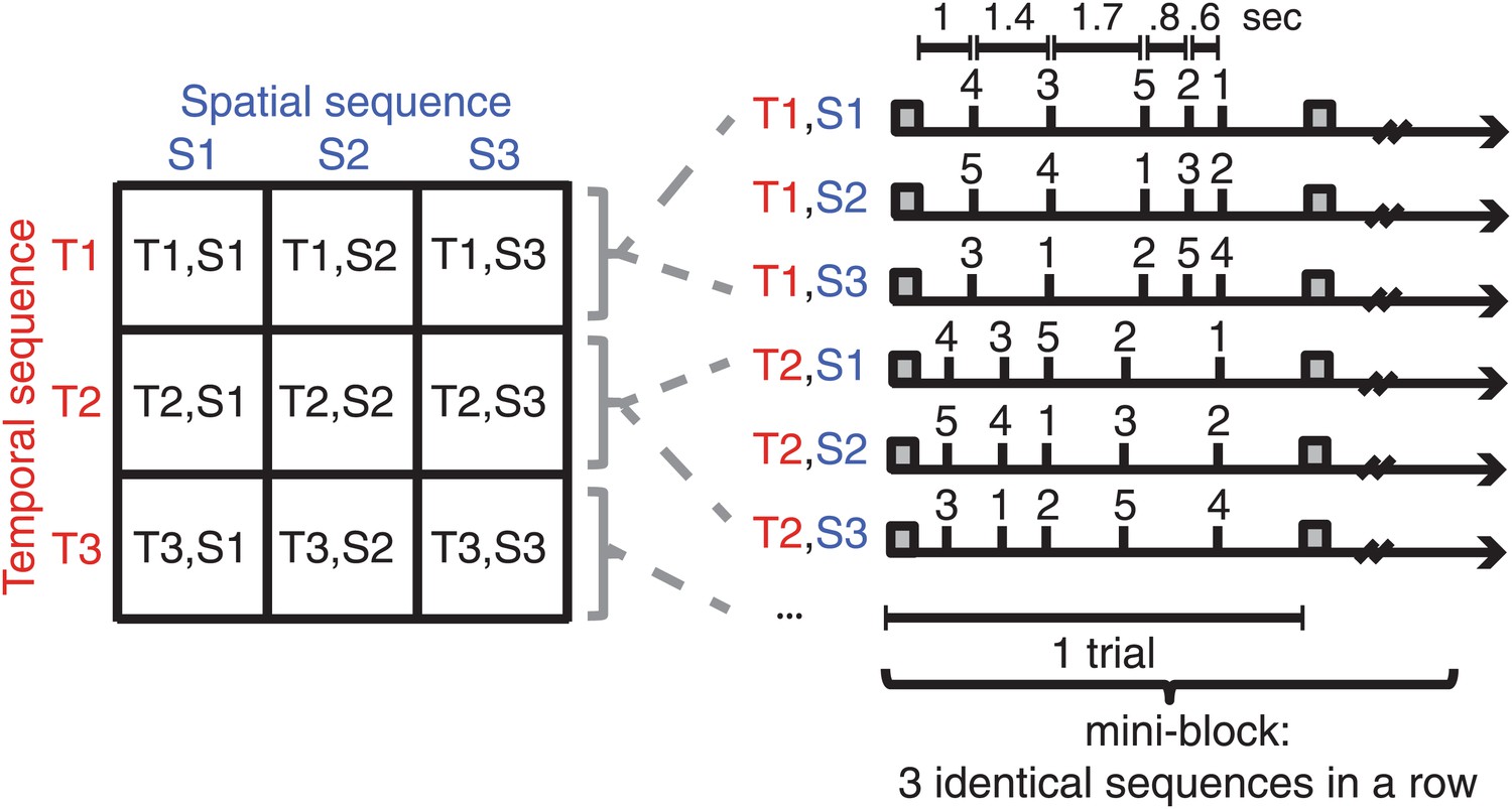
Subjects were trained on nine sequences, which were unique combinations of three spatial (finger order) and three temporal sequence features.
Sequences were presented in mini-blocks of three trials in a row. Each sequence began with the presentation of a warning cue (square).
Figure 2 with 1 supplement
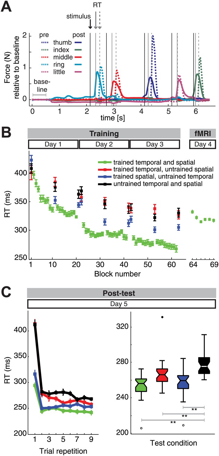
Reaction time (RT) results.
(A) Two trial examples of force traces show faster finger responses to visual stimuli after (‘post’) as opposed to the beginning of training (‘pre’). (B) Subjects showed general and sequence-specific learning during the training of the combined temporal and spatial sequences. The RT remained relatively stable across the fMRI session runs, albeit overall higher than at the end of training outside the MRI environment. (C) Post-test results. Left panel: repeating sequences nine times in the test phase yielded an immediate RT decrease for trained spatial sequences (blue) relative to untrained sequences (black), and only delayed RT differences for trained temporal sequences (red), in line with previous results (Kornysheva et al., 2013). Right panel: a boxplot displaying RT results across subjects and all sequence repetitions in the post-test revealed significant RT advantages for the trained sequence, as well as the trained spatial and trained temporal feature conditions when compared to untrained sequences, suggesting that both the finger order and their relative timing were represented independently. A double asterisk (**) indicates a significant difference between conditions with p<0.01. Errorbars in the lineplots and maximum and minimum RTs (boxplot whiskers) are corrected for differences in the mean RT across individuals, and therefore represent the interindividual variability of relative RT differences across conditions. In the boxplot, upper and lower edges signify the 75th (third quartile) and 25th percentile (first quartile), respectively. The median is designated as a horizontal white or black line in the box. Outliers (equal or above 3*interquartile range above the third quartile or below the first quartile) are depicted as filled circles, suspected outliers (1.5*interquartile range above the third quartile and below the first quartile) are depicted as unfilled circles, respectively.
Figure 2—figure supplement 1
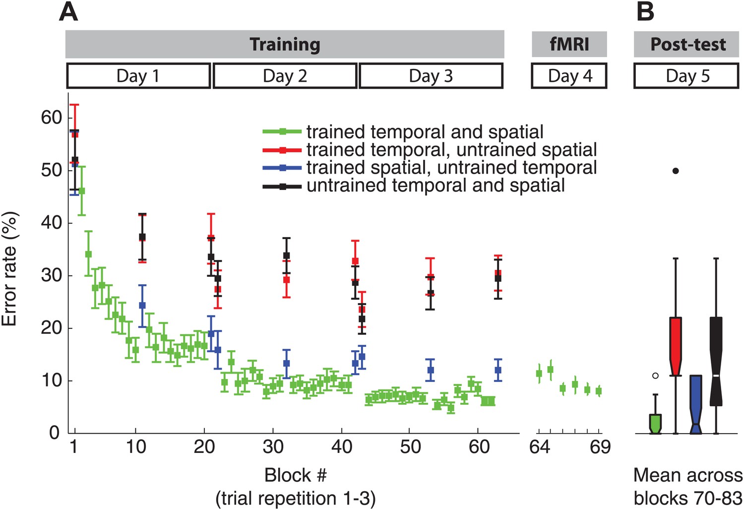
Error rate paralleled the RT results during the training (A) and fMRI showing clear sequence-specific advantages for the trained sequences, as well as sequences which retained the spatial features.
Note that in contrast to the RT results in Figure 2C, the post-test (B) did not show a decrease of error rate for sequences with trained temporal, but new spatial features consistent with our previous behavioural findings (Kornysheva et al., 2013).
Figure 3
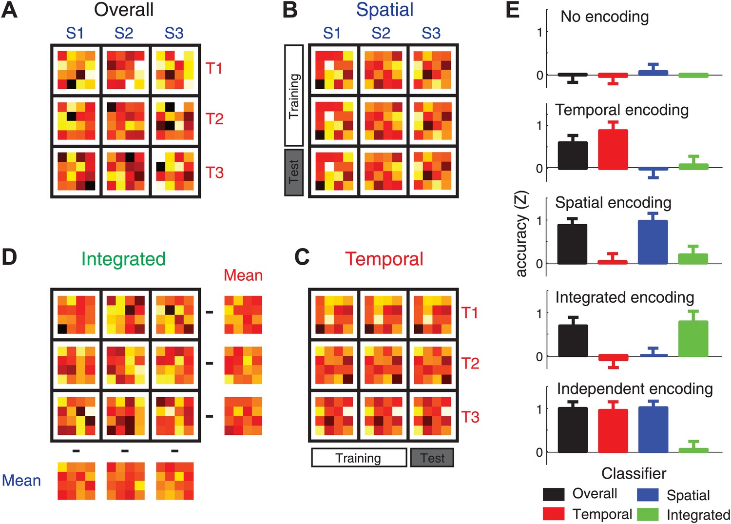
Four classification procedures were employed to classify the voxel pattern of each searchlight (160 voxels, here reduced to 16 units for illustration purposes).
(A) To test whether a voxel searchlight contained any sequential information, the overall classifier distinguished between the nine sequences independently. Classification was always cross-validated across imaging runs (‘Materials and methods’). (B) To determine encoding of the spatial feature, the classifier was trained on data involving only two of the three temporal sequences, and tested on trials from a left-out imaging run in which the spatial sequences were paired with the remaining temporal sequence. (C) The temporal classifier followed the same training-test principle, but in an orthogonal direction. (D) The integrated classifier detected nonlinear encoding of the unique combinations of temporal and spatial features that could not be accounted for by linear superposition of independent encoding. The spatial and temporal mean patterns for each run were subtracted from each combination, respectively, to yield a residual pattern, which was then submitted to a nine-class classification. (E) Classification accuracy of the four classifiers on simulated patterns (z-transformed, chance level = 0). Results indicate that the underlying representation can be sensitively detected by contrasting the overall, temporal, spatial, and integrated classifiers. Importantly these classification procedures can differentiate between a non-linear integrated encoding of the two parameters as opposed to the overlap of independent temporal and spatial encoding.
Figure 4 with 4 supplements
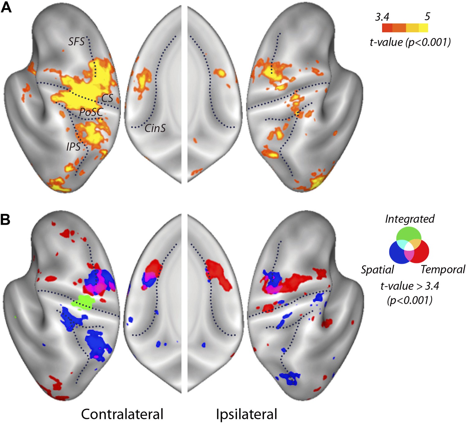
Searchlight classification results shown on an inflated representation of the cortical surface.
(A) Group t-values indicate regions in which the overall classifier performed significantly above chance. (B) Significant group-level above chance classification of spatial (blue), temporal (red), and integrated (green) classifiers. Results are presented at an uncorrected threshold of t(31) > 3.37. p<0.001. CinS, cingulate sulcus; CS, central sulcus; IPS, intraparietal sulcus; PoSC, postcentral sulcus; SFS, superior frontal sulcus.
Figure 4—figure supplement 1
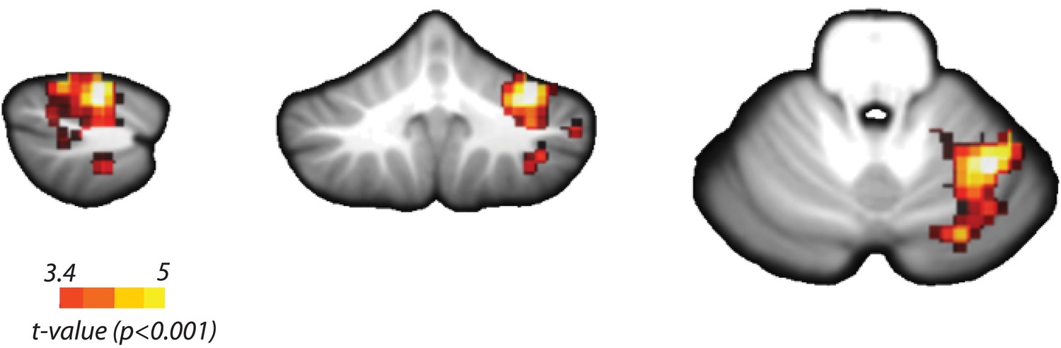
Searchlight classification results in the cerebellum.
Yellow scale indicates consistent above chance classification across the group by the overall classifier in ipsilateral Lobules V/VI (Peak t(31) = 5.72, pcluster<0.001, MNI coordinates: 34, −54, −23). Temporal, spatial, and integrated classifiers did not show significant encoding at an uncorrected threshold of t(31) > 3.37, p<0.001.
Figure 4—figure supplement 2
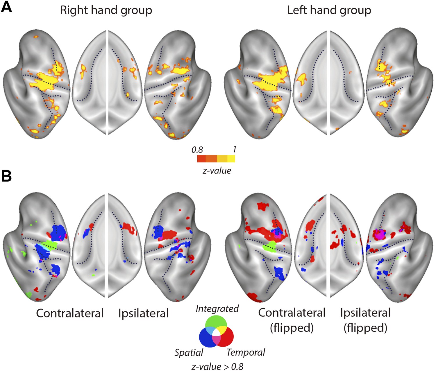
Mean searchlight classification accuracy results displayed as in Figure 4, split by group trained on the right and left hand.
(A) Classification accuracy results (z-values). Yellow scale indicates above chance classification by the overall classifier. Results are presented a threshold of z = 0.8 (chance level: z = 0). (B) Blue, red, and green colours stand for above chance classification of spatial, temporal, and integrated patterns, respectively.
Figure 4—figure supplement 3
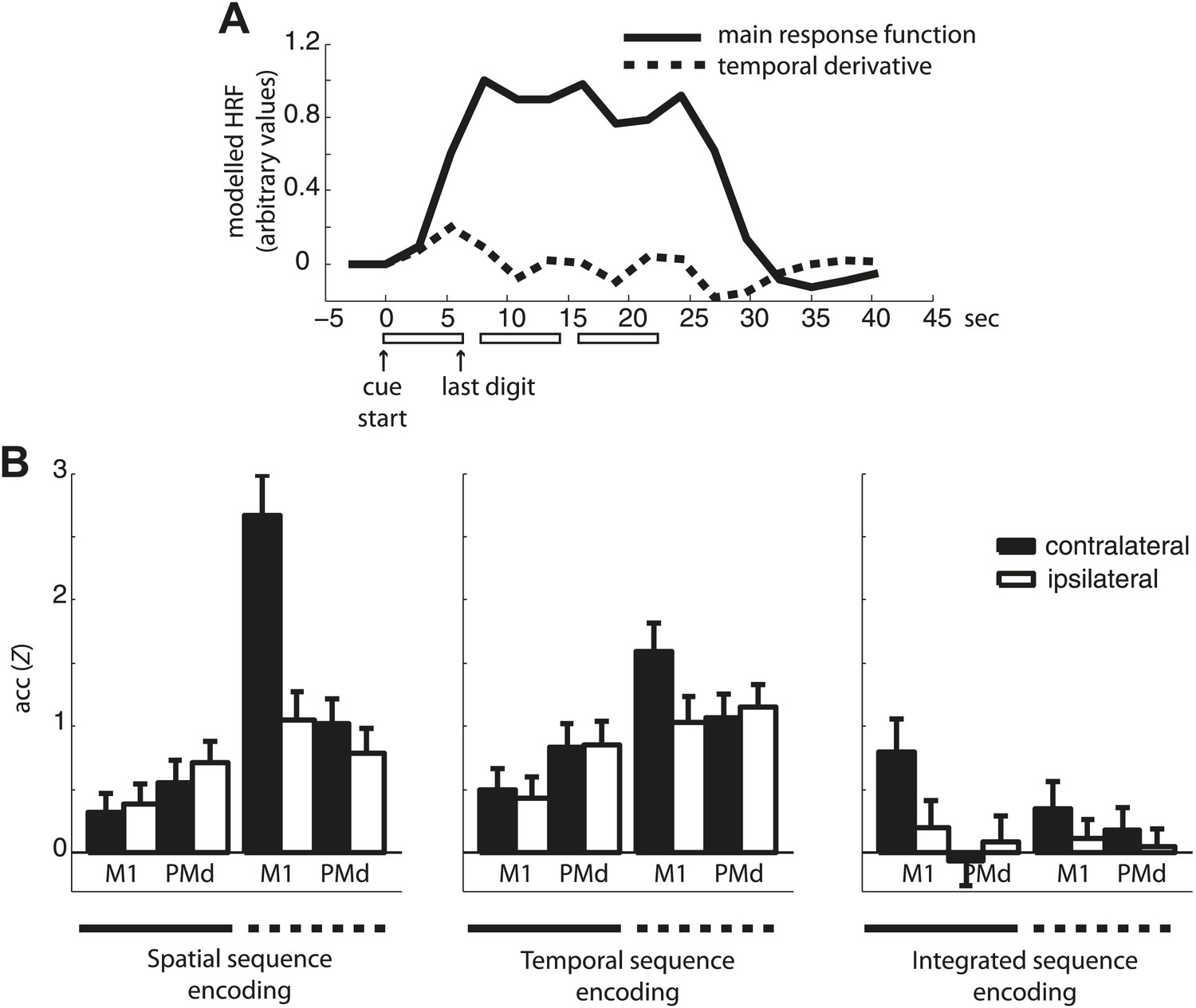
Classification accuracy of the main response function and temporal derivative.
(A) An example of the main response function and temporal derivative for three sequence repetitions (one mini-block). Note that in contrast to the temporal derivative that captures the temporal evolution of each sequence by returning to baseline between each sequence, the main response function used in the subsequent classification analysis remains elevated across the three sequence repetitions. (B) Classification accuracy of the main response vs the temporal derivative estimates in contra- and ipsilateral M1 and PMd.
Figure 4—figure supplement 4
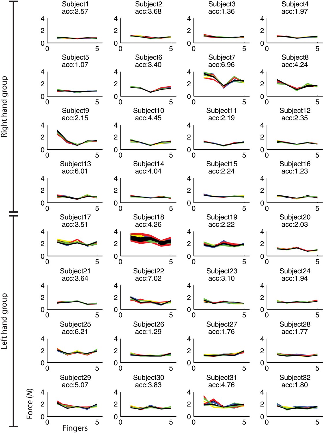
Maximum force for finger 1(thumb) to 5 (pinkie) during fMRI.
Each line depicts each participant's mean force across fingers for each of the nine trained sequences. Sequence specific idiosyncratic force profiles could be used to classify the sequences above chance (p<0.001; acc: z-transformed accuracy, chance level = 0).
Figure 5 with 1 supplement

Classification accuracy (z-values) in anatomically and symmetrically defined motor regions of interest (ROI).
Integrated classification accuracy was significant above chance level in contralateral M1 only, whereas temporal and spatial classifiers showed higher accuracy in premotor areas, in a partly overlapping manner.
Figure 5—figure supplement 1
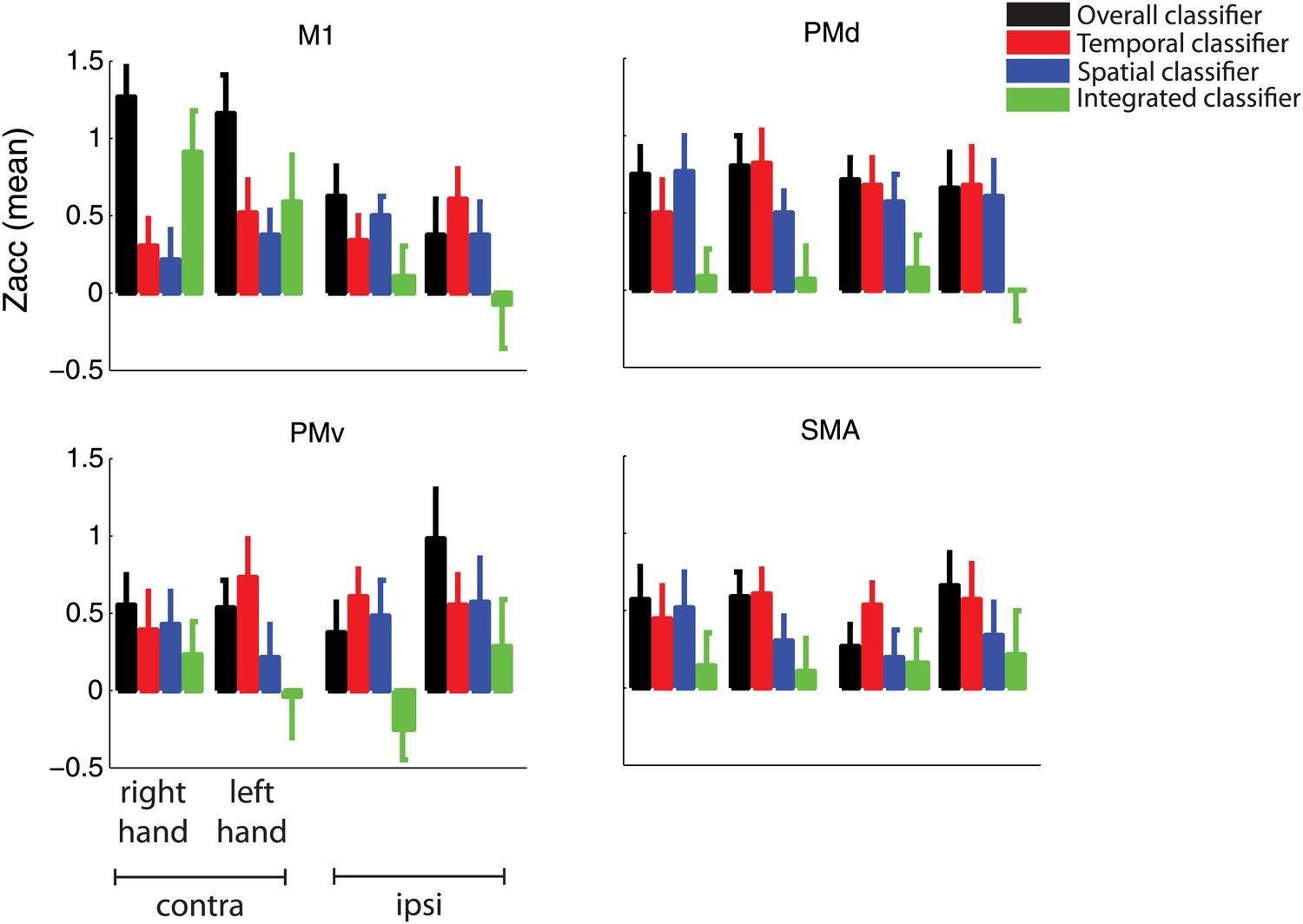
Classification accuracy as in Figure 5 split by group trained on the right and left hand.
https://doi.org/10.7554/eLife.03043.014
Figure 6 with 1 supplement
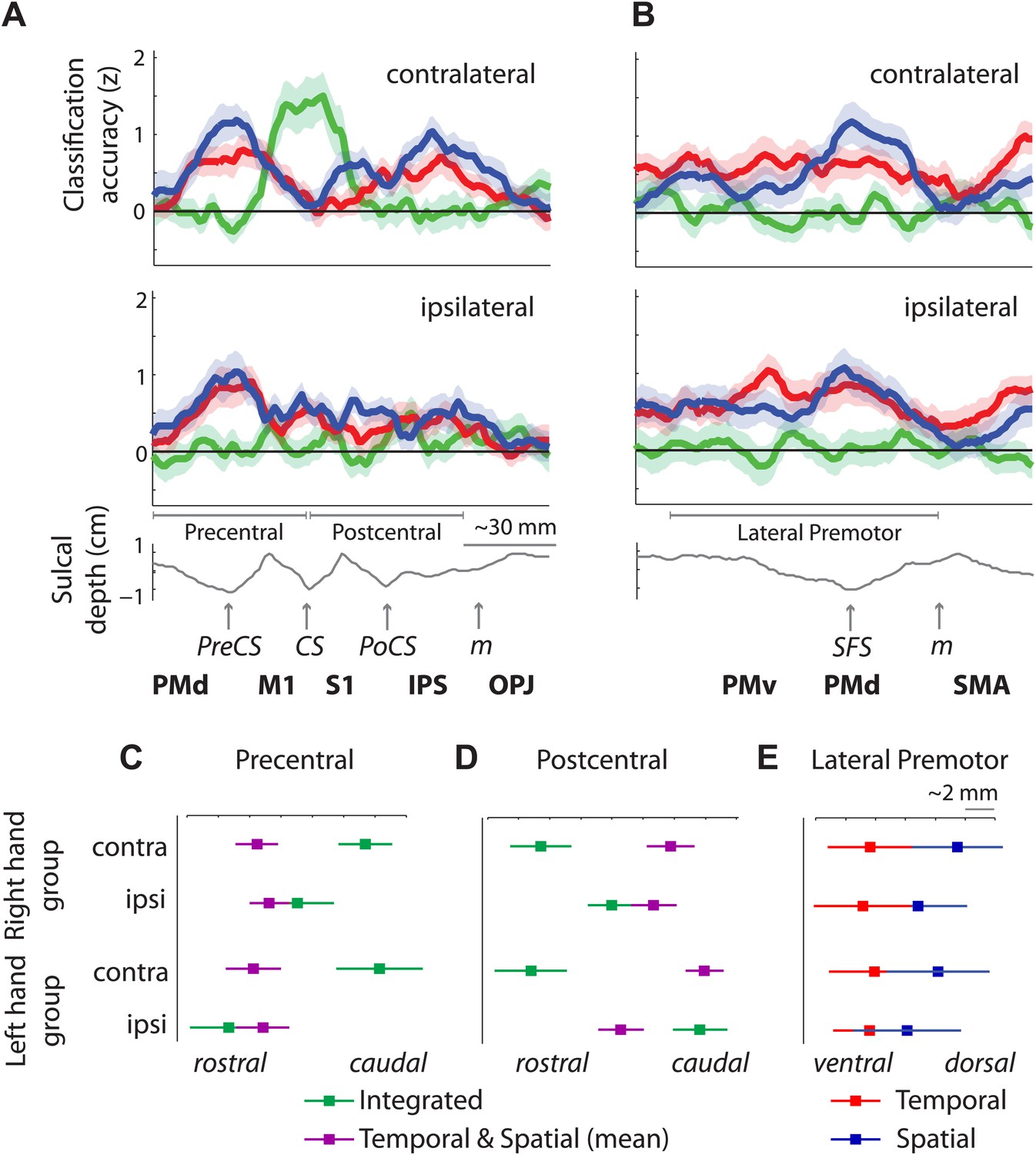
Distribution of encoding in cortical cross-sections.
Shown are profiles of integrated (green), temporal (red), and spatial (blue) classification accuracy (z-values), (A) on a cross-section running from rostral premotor cortex, through the hand area, to the occipito-parietal junction and (B) on a profile running from the ventral, through the dorsal premotor cortex, to the SMA (BA 6). (C) Center of gravity (CoG) analysis across the precentral part (between rostral PMd and central sulcus) of the profile in A shows that independent temporal and spatial classification accuracy (mean in purple) is represented more rostrally to integrated classification accuracy in the contralateral hemisphere across right and left hand groups. (D) CoG analysis across the postcentral part of the profile shows the opposite pattern to C with independent classification accuracy represented more caudally, further away from the CS towards the parietal cortex as compared to integrated classification accuracy. This gradient was found in the contralateral hemisphere across right and left hand groups. (E) CoG analysis across the lateral premotor cortex shows a slight ventral bias for temporal compared to spatial classification accuracy across hemispheres and groups. BA, Brodmann area; CoG, center of gravity; IPS, inferior parietal sulcus; m, medial wall; M1, primary motor cortex; OPJ, occipito-parietal junction; PMd, dorsal premotor cortex; PMv, ventral premotor cortex; PoCS, postcentral sulcus; PreCS, precentral sulcus ventral premotor cortex; S1, primary sensory cortex; SFS, superior frontal sulcus; SMA, supplementary motor area.
Figure 6—figure supplement 1
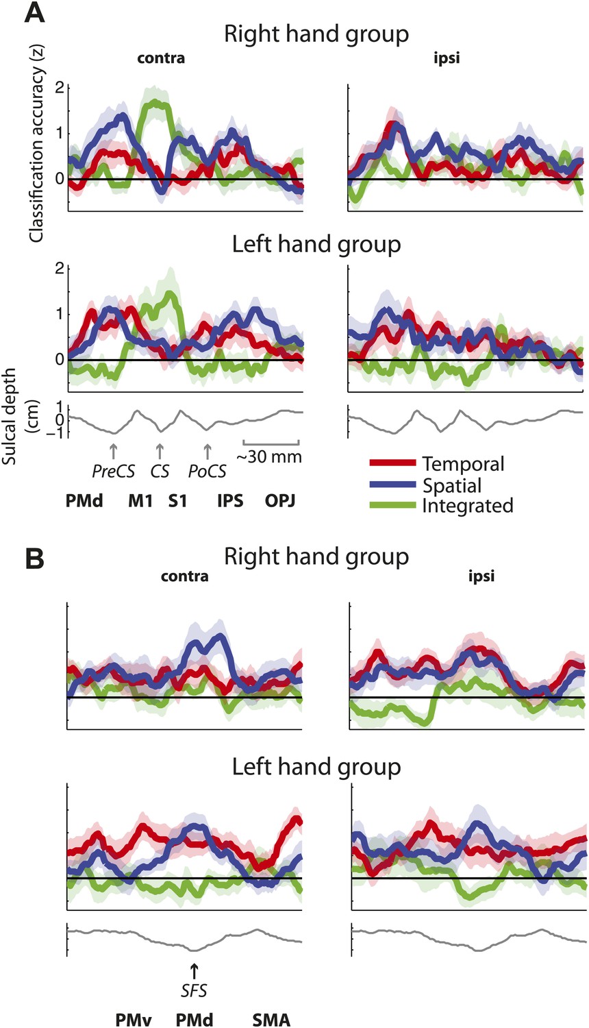
Distribution of encoding as in Figure 6 split by group (A) on a cross-section running from rostral premotor cortex, through the hand area, to the occipito-parietal junction and (B) on a cross-section running from the ventral, through the dorsal premotor cortex, to the SMA (BA 6).
https://doi.org/10.7554/eLife.03043.016
Figure 7
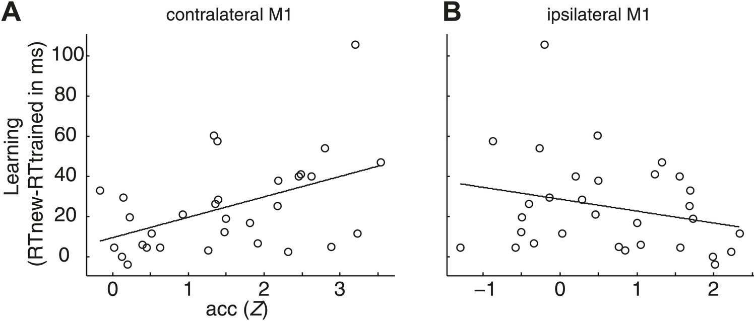
Correlation between sequence-specific learning (RT advantages for trained relative to untrained sequences in the post-test) and overall encoding in M1.
Learning significantly covaried with the overall encoding in the contralateral M1 r = 0.47, p=0.008 (A), but not in the ipsilateral M1 r = −0.25, p=0.169 (B). The correlation of sequence learning and contralateral encoding in M1 remained significant when taking all, and not only the task-activated voxels in contralateral M1 into account, (r = 0.369, p=0.041).
Tables
Table 1
Areas showing above-chance classification accuracy for the decoding of sequences and their spatial and temporal features
| MNI | |||||||
|---|---|---|---|---|---|---|---|
| Classifier | Area (Brodmann area) | Area (cm2) | Pcluster | Peak t(31) | X | Y | Z |
| Overall | Contralateral | ||||||
| M1/PMd/PMv (BA4/BA6) | 43.25 | <0.001 | 9.40 | −36 | −22 | 53 | |
| Superior parietal (BA40/BA7) | 15.80 | <0.001 | 5.82 | −32 | −54 | 56 | |
| Extrastriate vis cortex (BA18) | 8.53 | <0.001 | 5.75 | −27 | −90 | −1 | |
| Extrastriate vis cortex (BA19) | 2.35 | 0.002 | 5.57 | −36 | −83 | 27 | |
| SMA (BA6) | 3.86 | <0.001 | 5.27 | −8 | −12 | 57 | |
| 2.22 | 0.002 | 4.73 | −42 | −82 | −13 | ||
| Anterior insula (BA48) | 1.35 | 0.036 | 4.35 | −35 | −10 | −2 | |
| 1.81 | 0.008 | 4.32 | −42 | 2 | 12 | ||
| Occipitotemporal area (BA37) | 1.75 | 0.01 | 4.10 | −40 | −62 | −11 | |
| Ipsilateral | |||||||
| Extrastriate vis cortex (BA19) | 20.84 | <0.001 | 5.77 | 34 | −89 | −6 | |
| PMd (BA6) | 12.72 | <0.001 | 5.24 | 21 | −12 | 60 | |
| Superior parietal (BA5) | 3.76 | <0.001 | 5.19 | 19 | −55 | 61 | |
| Superior parietal (BA7) | 3.27 | <0.001 | 4.92 | 30 | −59 | 46 | |
| Medial M1 (BA4) | 4.84 | <0.001 | 4.86 | 14 | −40 | 59 | |
| Occipitotemporal area (BA37) | 1.83 | 0.014 | 4.55 | 45 | −70 | 6 | |
| Extrastriate vis cortex (BA19) | 2.55 | 0.002 | 4.22 | 32 | −75 | −11 | |
| SMA/Pre-SMA (BA6/BA32) | 1.39 | 0.05 | 3.93 | 8 | 18 | 49 | |
| Integrated | Contralateral | ||||||
| M1 (handknob, BA4) | 5.89 | <0.001 | 5.39 | −33 | −23 | 59 | |
| Spatial | Contralateral | ||||||
| Superior parietal (BA7) | 10.00 | <0.001 | 6.93 | −31 | −56 | 60 | |
| PMd (BA6) | 9.66 | <0.001 | 6.20 | −31 | −13 | 53 | |
| Inferior parietal (BA40) | 6.00 | <0.001 | 5.78 | −39 | −36 | 37 | |
| SMA (BA6) | 2.69 | 0.002 | 5.70 | −9 | 1 | 54 | |
| Ipsilateral | |||||||
| PMd (BA6) | 5.23 | <0.001 | 4.68 | 29 | −2 | 47 | |
| Inferior parietal/occipital | 3.98 | <0.001 | 4.31 | 33 | −66 | 34 | |
| (BA39/BA19) | |||||||
| Temporal | Contralateral | ||||||
| SMA (BA6) | 3.47 | <0.001 | 5.74 | −8 | 9 | 48 | |
| PMd (rostral BA6) | 6.38 | <0.001 | 5.53 | −24 | −15 | 58 | |
| Extrastriate vis cortex (BA18) | 11.00 | <0.001 | 4.58 | −29 | −92 | −5 | |
| Extrastriate vis cortex (BA19) | 2.35 | 0.006 | 4.34 | −35 | −82 | 10 | |
| Ipsilateral | |||||||
| PMd (rostral, BA6) | 9.78 | <0.001 | 5.98 | 23 | −9 | 49 | |
| PMv (BA6) | 5.19 | <0.001 | 5.28 | 51 | −6 | 24 | |
| Posterior cingulate (BA23) | 2.44 | 0.006 | 4.83 | 9 | −30 | 31 | |
| Pre-SMA/anterior cingulate | 2.73 | 0.004 | 4.79 | 9 | 34 | 42 | |
| (BA32) | |||||||
| PMd (caudal BA6) | 1.75 | 0.034 | 4.66 | 20 | −26 | 57 | |
| Extrastriate vis cortex (BA19) | 1.75 | 0.034 | 4.13 | 42 | −85 | 1 | |
-
Results of surface-based random effects analysis (N = 32) with an uncorrected threshold of t(31) > 3.37, p<0.001. p (cluster.) is the cluster-wise p-value for the cluster of that size. The p-value is corrected over the cortical surface using the area of the cluster (Worsley et al., 1996). The cluster coordinates reflect the location of the cluster peak in MNI space.
Additional files
-
Source code 1
Custom written multiclass classification function in Matlab which uses linear discriminant analysis.
Based on a training data set (such as beta values of runs 1–5 in a region of voxels) where the class identity is known, this classification function predicts the respective class identity of each datapoint in a test set (beta values of run 6 in the same region of voxels), for example, a unique combination of spatial and temporal sequence features in a sequence. Following training-test cross-validation (‘Materials and methods’) the accuracy can be determined by computing the percentage of datapoints that were classified correctly.
- https://doi.org/10.7554/eLife.03043.018
Download links
A two-part list of links to download the article, or parts of the article, in various formats.
Downloads (link to download the article as PDF)
Open citations (links to open the citations from this article in various online reference manager services)
Cite this article (links to download the citations from this article in formats compatible with various reference manager tools)
Human premotor areas parse sequences into their spatial and temporal features
eLife 3:e03043.
https://doi.org/10.7554/eLife.03043


