Texture coarseness responsive neurons and their mapping in layer 2–3 of the rat barrel cortex in vivo
- The Rappaport Faculty of Medicine and Research Institute, Technion-Israel Institute of Technology, Israel
- Ben-Gurion University of the Negev, Israel
Figures
Figure 1 with 6 supplements
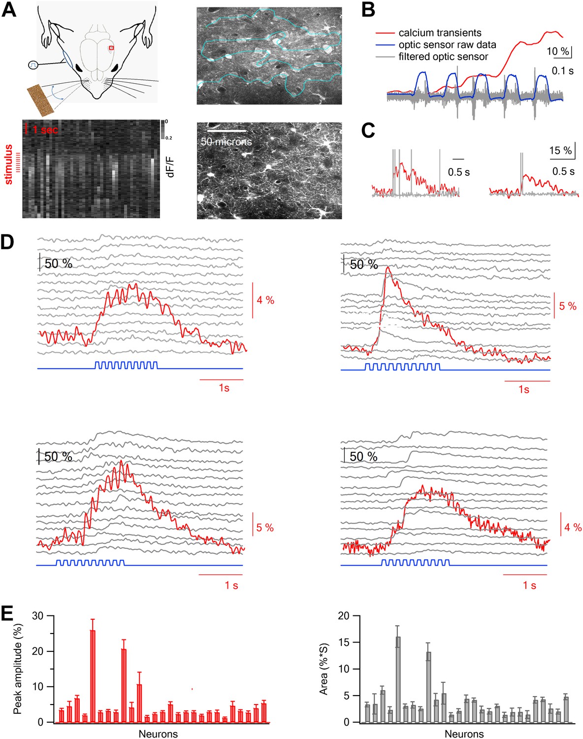
Two-photon calcium imaging of layer 2–3 neurons evoked by artificial whisking against textures in the barrel cortex in vivo.
(A) Experimental set-up. A small (2 × 2 mm) craniotomy was performed above the barrel cortex, and the dura was carefully removed. Nerve stimulation was performed with a silver hook attached electrode to the buccal nerve. Only the principle whisker was left intact while other whiskers were trimmed. Artificial whisking (10 trains at 5.5 Hz) was performed either in free air (FW) or against different sandpapers. The calcium indicator Fluo-4 AM and the astrocytic dye SR101 were injected to layer 2–3 via a glass pipette under visual control using the two-photon microscope. The right upper panel shows an image of all cells filled with Fluo-4 and the right lower panel shows the astrocytes filled with SR101 in the same field of view (260 µm from pia). Left lower panel, calcium dependent fluorescent signals were collected from cells (horizontal aspect) using the free hand line scan mode (cyan line in right upper panel) and presented as a function of time (vertical aspect). Red lines mark the stimulus time. (B) Simultaneous recordings of the fluorescent calcium signal (red) and whisker trajectory (gray and blue) recorded using an optic sensor. The blue trace shows the unfiltered optical signal, and the gray trace shows the same optical data filtered (band pass of 50–500 Hz). 10% scale bar denotes the ΔF/F calcium transient signal. (C) Simultaneous voltage recording (gray) and calcium imaging (red) from a single neuron. The cell was bulk loaded with Fluo-4 and electrophysiological recordings were performed in the cell-attached recording mode from visually targeted neurons. Action potentials were partially truncated in the electrophysiological traces. (D) Example of the averaged calcium transient (red) and the corresponding single traces (14 repetitions, gray) from 4 single cells are presented together with the whisker stimulation (blue, 10 whisking cycles at 5.5 Hz). The traces in the different neurons were obtained simultaneously in the free hand line-scan imaging mode. (E) Average peak amplitude (±SEM) (red) and area (gray) of the calcium transients evoked by artificial whisking for all the cells (n = 51) recorded in one experiment.
Figure 1—figure supplement 1
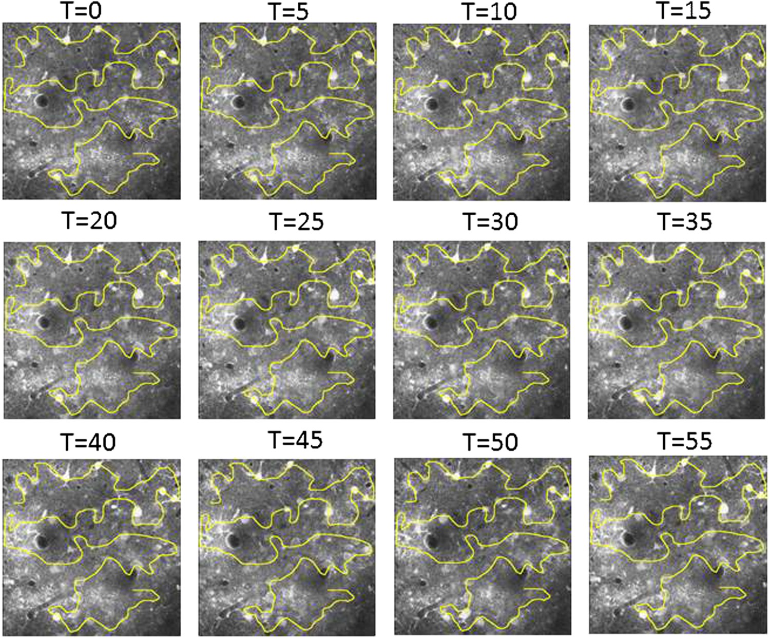
Free hand line scan position stability.
Example of control images acquired every 5 min to verify the location of the free hand line scan path relative to the neurons. If necessary the line scan path was corrected so the same neurons can be compared throughout the length of the experiment.
Figure 1—figure supplement 2
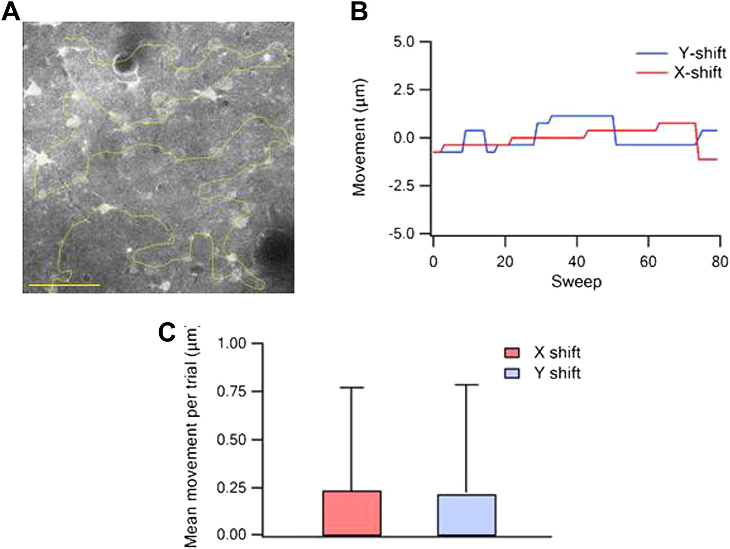
Quantification of the free hand line scan position stability.
(A) Example of a reference image of Fluo-4-labeled neurons with the scanned line passing through the neurons (yellow, scale bar 50 µm). (B) Measurements of X and Y image shifts compared to the reference image during all trails in a single experiment. (C) Average shift per trial (+SD) of the image in the X and Y directions (n = 15).
Figure 1—figure supplement 3
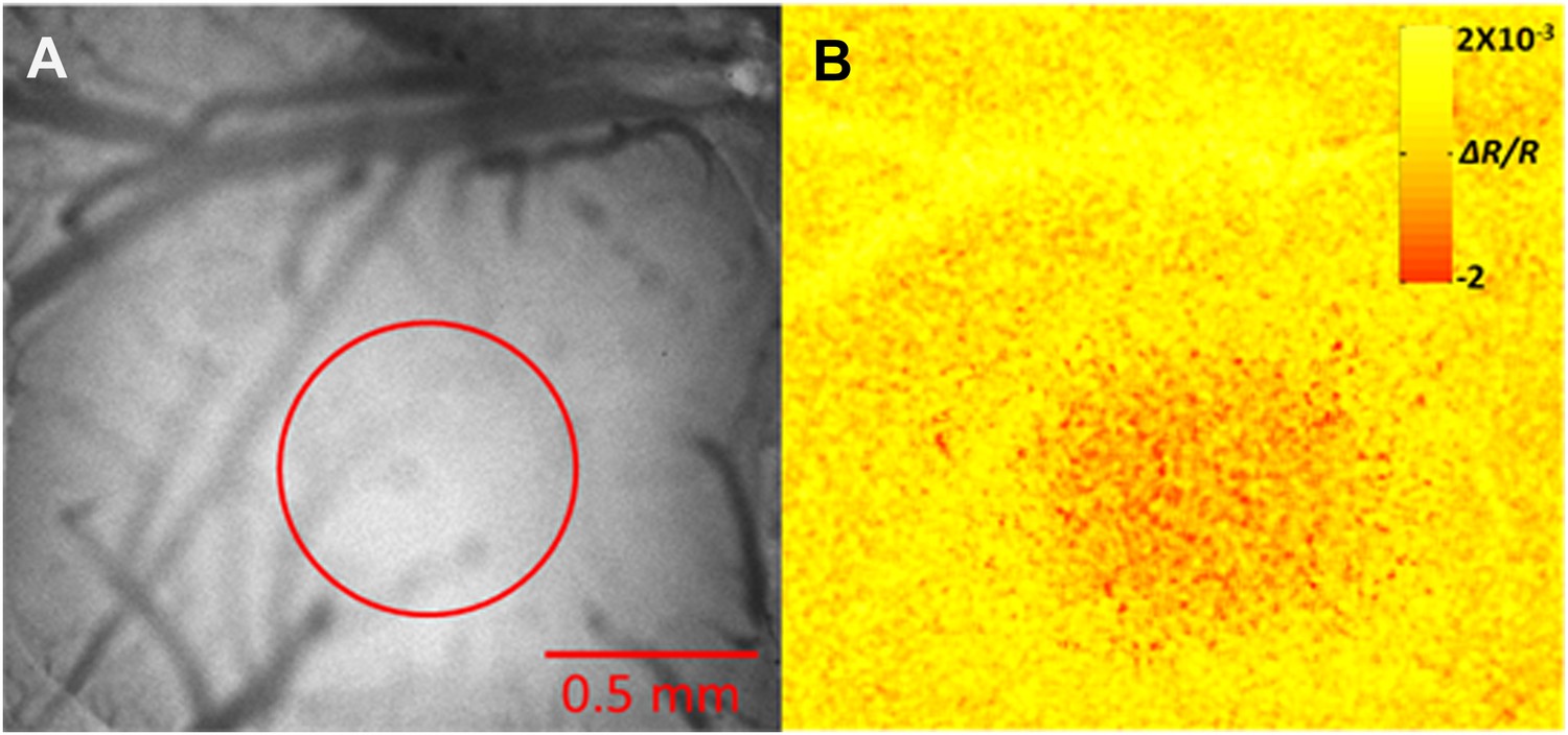
Intrinsic optical imaging mapping of the principle barrel.
(A) The bone above the barrel cortex was thinned and the surface blood vessels were imaged. (B) Intrinsic optical imaging (610-nm LED) shows a decrease in the reflectance during stimulation of whisker D2 in this example (6 Hz deflections over 2 s duration). Red circle marks the region where decrease in reflectance was observed.
Figure 1—figure supplement 4
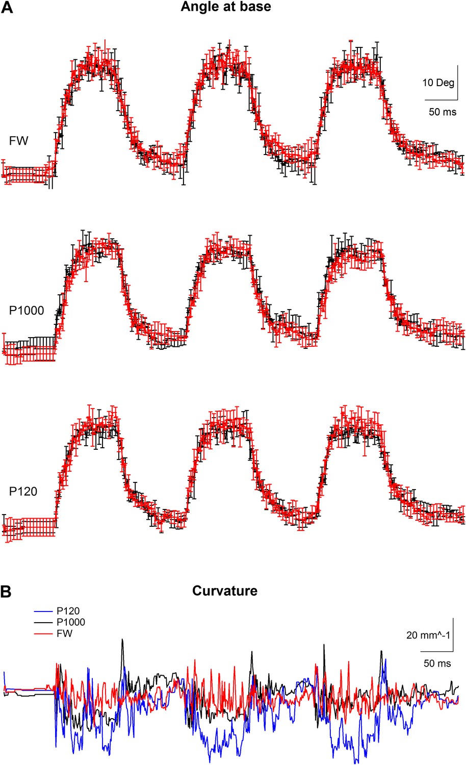
Kinematic variables of a whisker movement in artificially whisking rat.
(A) The angle at base of the whisker (mean ± SEM) during artificial whisking against free air (FW) and two different sandpapers, the finest (P1000) and the coarseset we used (P120). Whisker was photographed at 1000 Hz. Three individual artificial whisking trains were performed in two separate stimulation blocks, each composed of five consecutive repetitions. The average (±SEM) of the two whisking blocks is presented separately (red and black traces). The SEM is shown for every fifth point. (B) Average curvature calculated from the 10 repetitions for the three different conditions recorded (P120-blue, P1000-black, and FW-red).
Figure 1—figure supplement 5
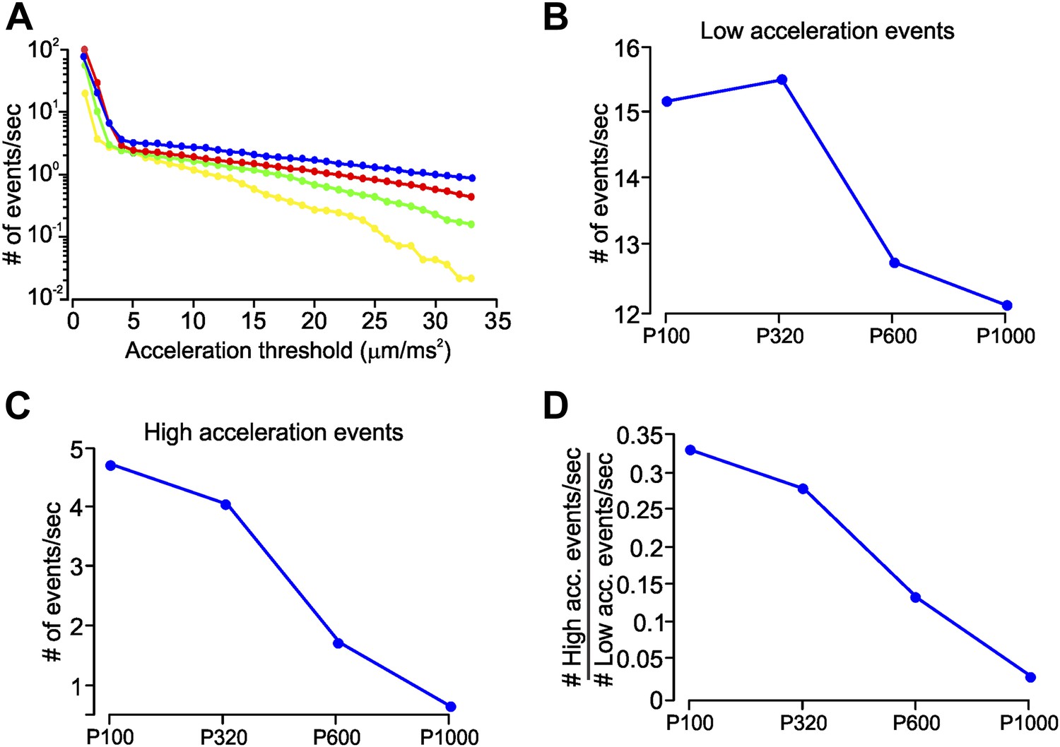
Slip-stick events characteristic to different coarseness.
(A) Mean number of acceleration events per second during whisker movement on four sandpapers (P120-blue, P320-red, P600-green, P1000-yellow), calculated on C3 whisker. Number of events per second is plotted on a log scale. Each point shows the cumulative number of events with acceleration greater than the threshold indicated on the x-axis. (B) Number of low-acceleration events (events with acceleration in the range 4–9 µm/ms2) measured on four textures. (C) Number of high-acceleration events (≥28 mm/ms2) across four textures. (D) Ratio of the number of high- to low-acceleration events per second, as a function of texture roughness.
Figure 1—figure supplement 6
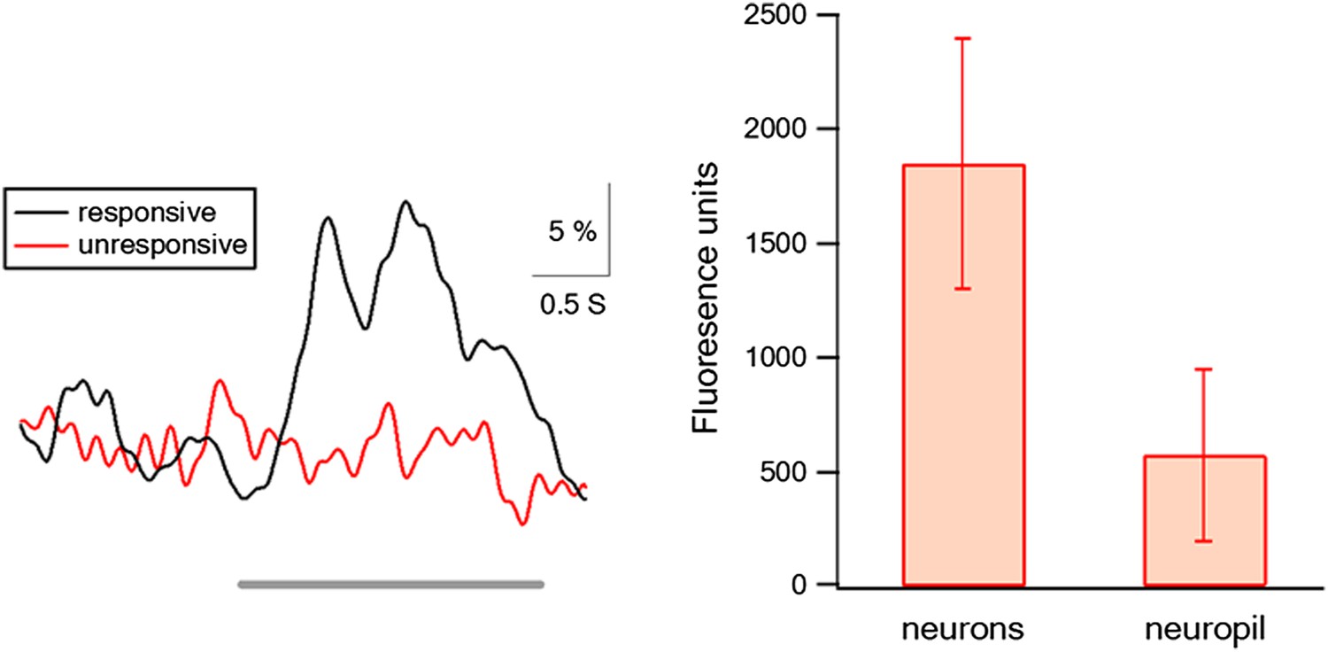
The relative fluorescence contributed from neuropil and out of focus signals.
Left panel shows the average transients of traces with and without action potential firing in the neurons in which we recorded simultaneously both electrophysiological and imaging data (n = 6). Traces without action potential firing represented the contribution of the neighboring out of focus neurons and neuropil signals, gray line represents stimulus time. Right panel shows the net fluorescence value (after background subtraction) in cells and in neuropil. Background was measured in neighboring blood vessels.
Figure 2 with 1 supplement
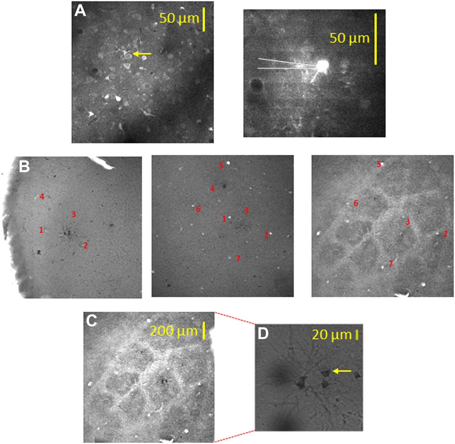
Alignment of the bulk loaded neurons in the TPLSM with the cytochrome oxidase barrel staining using biocytin electroporation of single neurons.
(A) TPLSM Fluo-4 bulk loaded image of the imaged field. At the end of the recording session single cell electroporation of biocytin was performed on the bulk loaded neurons (typically, 1–4 calcium loaded neurons). Yellow arrow point to the one of the electroporated cells (right panel). These biocytin electroporated neurons served as a definite marker to the location of the calcium bulk staining. (B) Brains were fixed and sliced (100 µm thick) at the tangential plane, and barrels were visualized according to the cytochrome oxidase dense regions typical to layer 4 barrels. Alignment of the neurons labeled with biocytin (in cortical layer 2–3) to the layer 4 cytochrome oxidase stained barrel according to identified ascending blood vessels (designated by numbers 1–7) in three consecutive slices from layer 2–3 to layer 4 (slices: 100–200 µm; 200–300 µm; 400–500 µm). (C) Superposition of the biocytin-labeled neurons onto the identified barrel in layer 4 (C2 in this example). (D) The biocytin-labeled neurons are shown in higher magnification (arrow point to the identified cell in A).
Figure 2—figure supplement 1
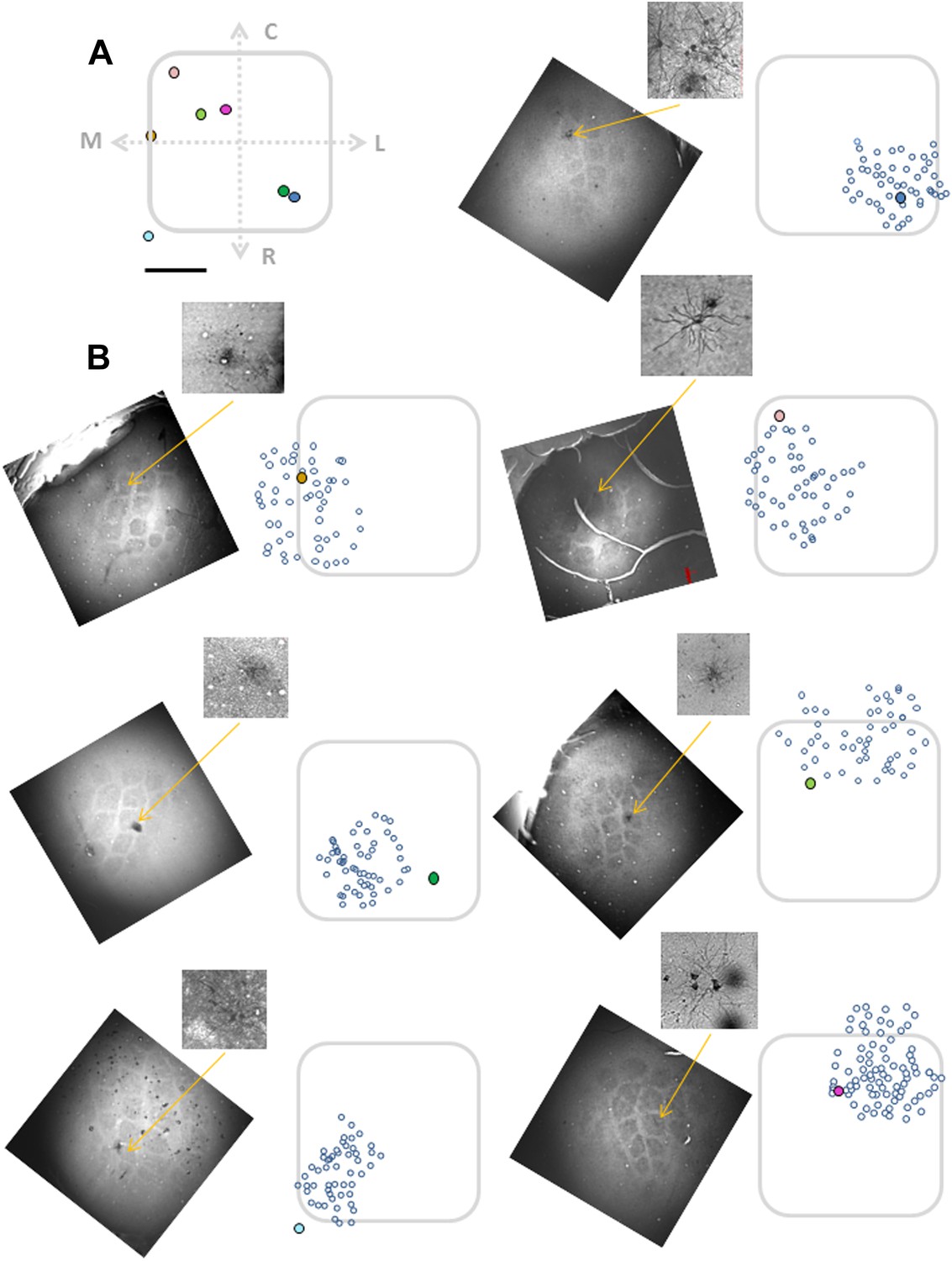
Alignment of the bulk loaded neurons onto the barrel using single elecrtoporated cells.
Top left panel (A) shows electroporated cells superimposed on a ‘normalized barrel’ in seven experiments (scale bare: 100 µm). Remaining seven panels (B) show the location of biocytine electroporated neurons (closed colorful circles) relative to the bulk loaded neurons (open circles) in seven individual experiments. Subset figures: the biocytin-labeled neurons are shown in higher magnification.
Figure 3 with 2 supplements
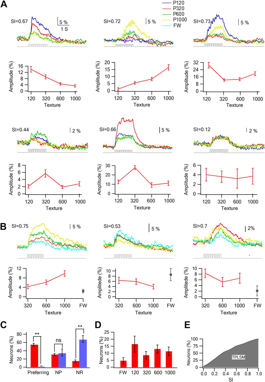
Texture preferring neurons in layer 2–3 barrel cortex evoked by artificial whisking: barrel vs septa regions.
(A) Examples of the average calcium transient responses (30 repetitions) of six neurons to different textures (upper panels) and their corresponding tuning curves (lower panels; mean ± SEM) as calculated from the peak of the averaged calcium response evoked by each texture. For each cell the selectivity index (SI) is calculated and presented in the upper left corner. P120-blue, P320-red, P600-green, P1000-yellow. (B) Examples of the average calcium transient responses (30 repetitions) of three neurons to different textures and free whisking (FW) and their corresponding tuning curves (lower panels; mean ± SEM) as calculated from the peak of the averaged calcium response evoked by each texture or FW. For each cell the selectivity index (SI) is calculated and presented in the upper left corner. P320-red, P600-green, P1000-yellow, and FW-cyan. (C) The percentage of neurons (out of 1158 neurons within barrel boundaries in 23 experiments; 301 neurons in septa in five experiments) that were either coarseness preferring, non-preferring (NP) or non-responsive (NR). Neurons were divided to those within the barrel boundaries (red) and those located in the septa regions (blue). (D) The coarseness preferring neuronal population (S.I. ≥ 0.35) was further subdivided according to their texture coarseness preference (either P1000, P600, P320, P120, or FW). (E) Cumulative histogram of S.I. (in percent values) calculated from the calcium transient signals of all responsive neurons.
Figure 3—figure supplement 1
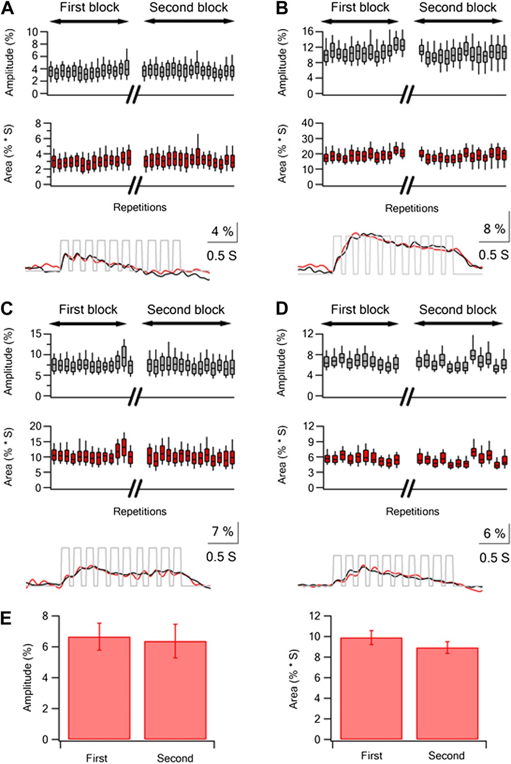
Repeated stimulation sessions of same textures resulted in reliable calcium responses in layer 2–3 neurons.
(A–D) Box plots of the peak amplitude (gray) and area (red) of the average calcium transients (mean ± SEM) in individual traces presented for different experiments (n = 4). The 30 traces were divided into two repetition blocks separated in time. In addition for each experiment the grand average calcium transient of all the neurons is presented for each repetition block (first black, second red) below the box plots. (E) The average (mean ± SEM; n = 5) peak amplitude (left panel) and area (right panel) of the grand averaged calcium responses during the first and second repetition blocks.
Figure 3—figure supplement 2
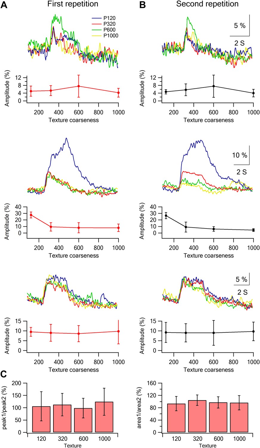
Stability of single neuron selectivity in repeated stimulation sessions.
(A and B) Examples from three neurons showing the tuning curves in the first (A, left) and second stimulation blocks (B, right). (C) Summary plot of the percent change (mean ± SD; n = 453 neurons) in the amplitude (left panel) and area (right panel) of the overall average calcium response between the two stimulation blocks. The data are shown for the response evoked by the four different textures.
Figure 4
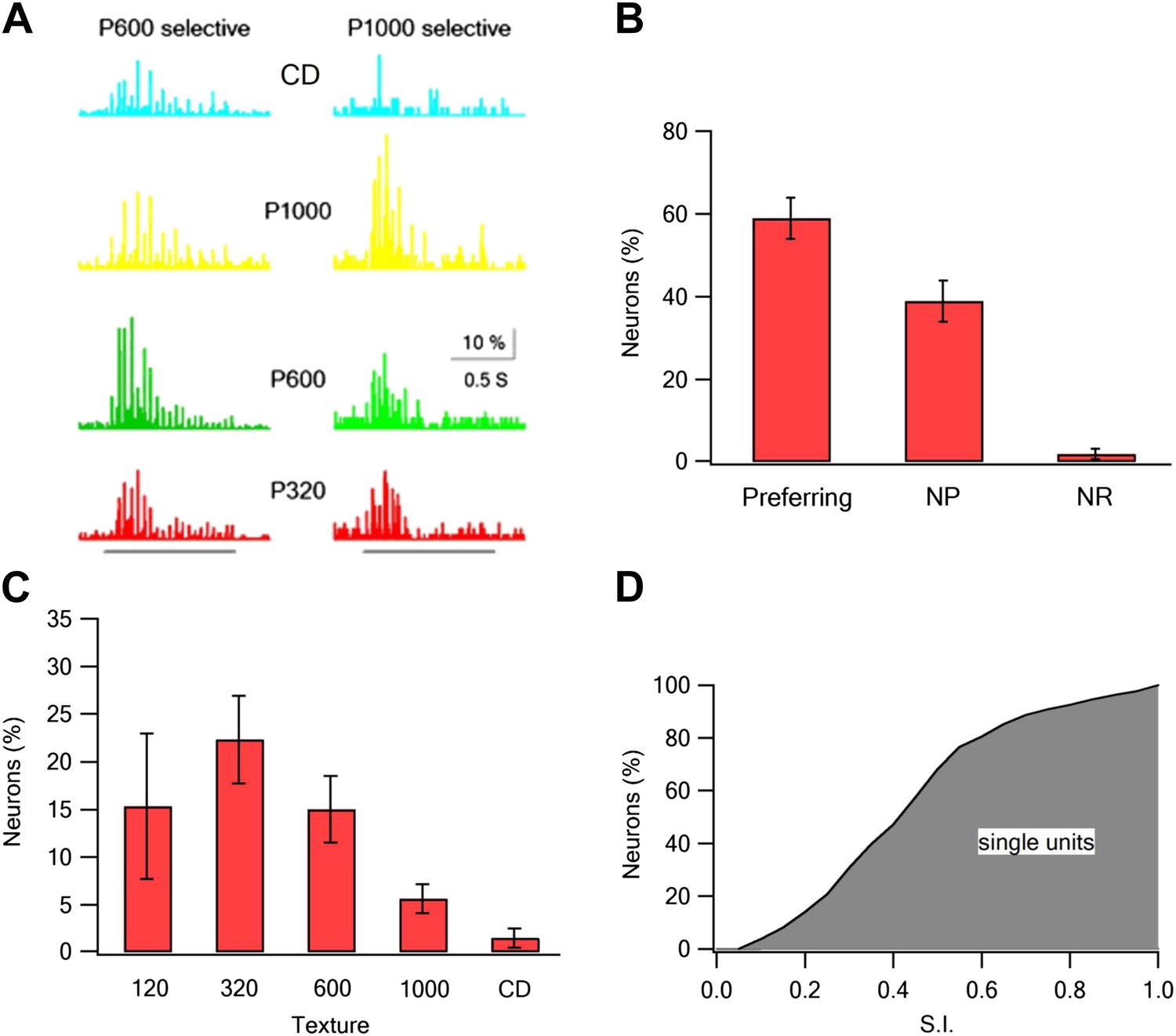
Coarseness preferring neurons as determined by extracellular single unit recordings.
Multi electrode single unit recordings were performed using multi-contact extracellular electrodes from the S1 barrel cortex. (A) Example of PSTHs from two neurons in response to different texture coarseness (CD, P320, P600 P1000). Each PSTH was acquired during artificial whisking (10 whisks applied at 5.5 Hz) against CD and three textures (P320, P600, and P1000). The responses of 170 consecutive artificial whisk trains are summed and presented in 10-ms time bins. The underlying gray line designates the time of whisking train. Note that the two neurons prefer different coarsenesses. The neuron presented on the right preferred the P1000 texture, while the neuron shown on the left prefer the P600 texture. (B) A summary of the responses acquired from single unit experiments (altogether 293 neurons from 19 rats). Responses were divided according to the percentage of neurons that were texture coarseness preferring (S.I. ≥ 0.35), non-preferring (NP; S.I. < 0.35) or non-responsive (NR) to all textures examined. (C) The coarseness preferring neurons were further subdivided to neurons that preferred either P1000, P600, P320, P120 textures or CD. (D) Cumulative histogram of S.I. calculated from the single unit recordings of all responsive neurons neurons.
Figure 5
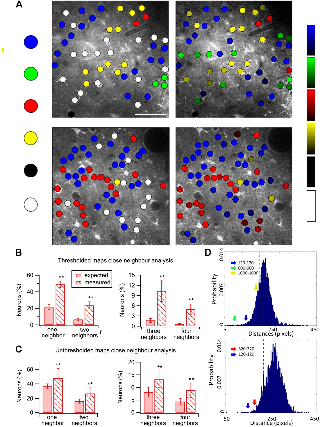
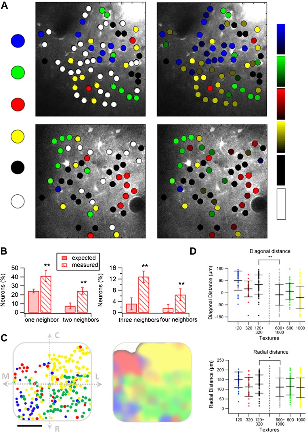
Spatial organization of texture preferring neurons during artificial whisking.
(A) Texture coarseness preferring neurons from two experiments (upper and lower panels) were color coded according to their preferred texture (P120-blue, P320-red, P600-green, P1000-yellow, non-preferring-white and non-responsive-black). Left panels: only cells with S.I. ≥ 0.35 were included (S.I. thresholded maps). Right panels: all responsive neurons (unthresholded maps) from the same two experiments were color coded according to their preferred texture and the selectivity strength (value of the S.I. is scaled for each color and presented on the right ranging from 0 to 1). (B and C) The probability of having 1, 2, 3, or 4 next neighbors with similar preferred textures was calculated for the thresholded maps (B) and unthresholded maps (C) and compared with the probabilities expected from random spatial distribution (n = 12 rats) (**p < 0.01). (D) Histograms of the Euclidian distance for 1000 runs for the two maps presented in A. To obtain these histograms the number of neurons that preferred each texture coarseness, as well as the number of non-responsive and non-preferring neurons was determined for each experiment. Later these neurons were randomly distributed in the recorded field 1000 times, and the Euclidian distance between neurons with the same preferred texture coarseness was measured. The broken line represents the lowest 5% of the histogram. The arrows represent the average experimental intra group distances for each texture coarseness (blue: P120-P120; red: P320-P320; green: P600-P600; yellow: P1000-P1000). Note that all intra-group distances in the two example experiments were below the 5% threshold value. The same result was obtained for all experiments tested (n = 20).
Figure 6 with 2 supplements
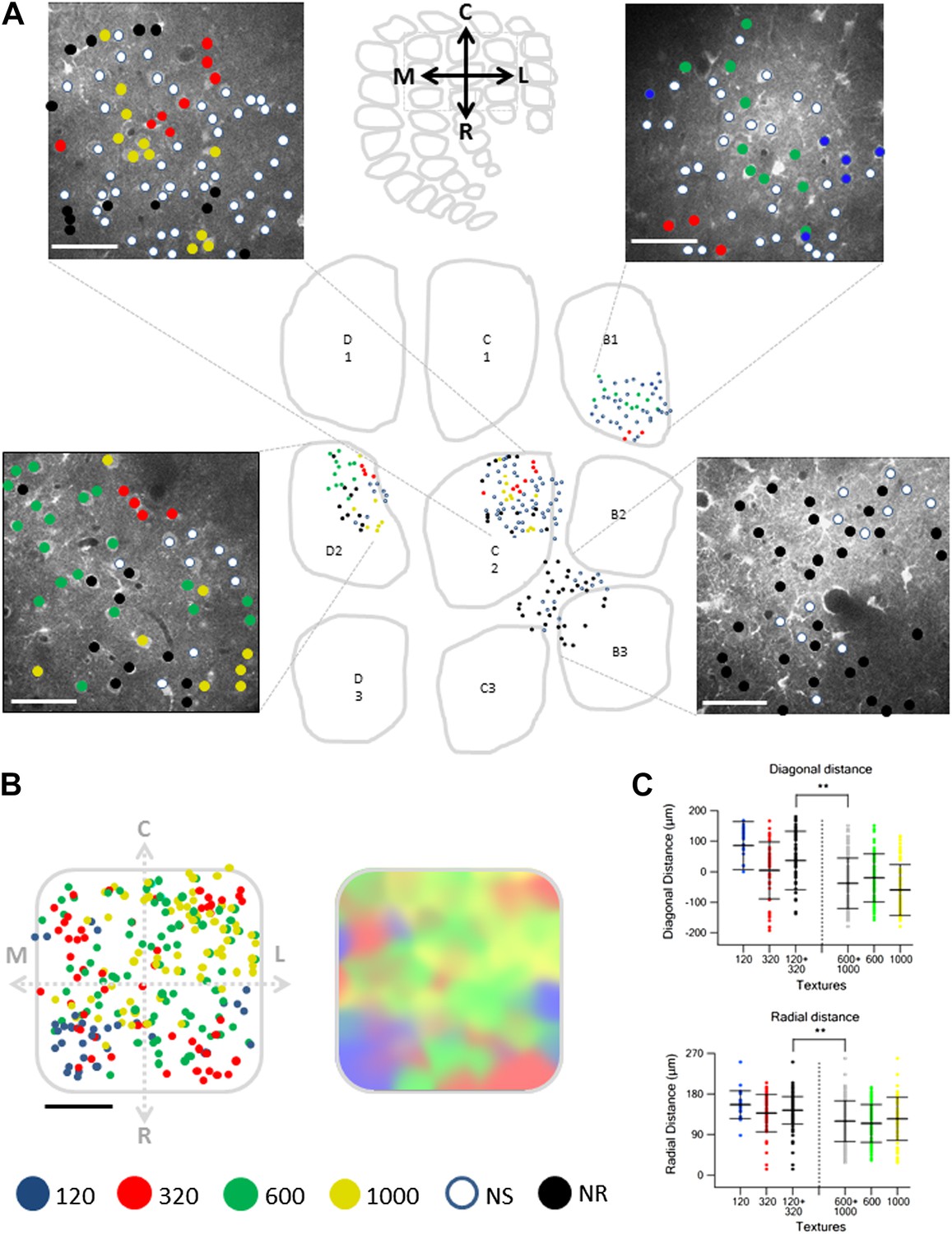
Spatial mapping of the preferred texture of neurons aligned to a normalized barrel.
(A) Examples of four spatial texture preference maps taken from four different brains (3 inside the barrel boundaries and 1 in the septa) are presented. We carefully aligned the neurons with the barrel field (Scale bar: 50 µm) (see Figure 2; ‘Materials and methods’ for details). (B) Left: superimposition of the spatial maps from 12 experiments onto a ‘normalized’ barrel (Scale bar: 100 µm), middle panel smoothened map. In 7 out of the 12 maps imaging location was determined using the electroporation method as described in Figure 2; in the remaining maps we used vertical blood vessels alignment. (The preferred textures of neurons were color coded as P120-blue originated from 6 rats, P320-red originated from 10 rats, P600-green originated from 8 rats, P1000-yellow originated from 10 rats, non-preferring-white and non-responsive-black.) (C) Distance from the MC-LR diagonal (upper) and radial distance from the center of the barrel (lower) of each cell in the different experiments is presented for each texture separately and for the combined coarser textures (black, P120 and P320) and finer textures (gray, P600 and P1000) (**p < 0.01 for comparison of coarser and finer textures). Comparison of the four textures with ANOVA was not significant for the radial distance and yielded a p < 0.01 for the distance from the MC-LR diagonal.
Figure 6—figure supplement 1
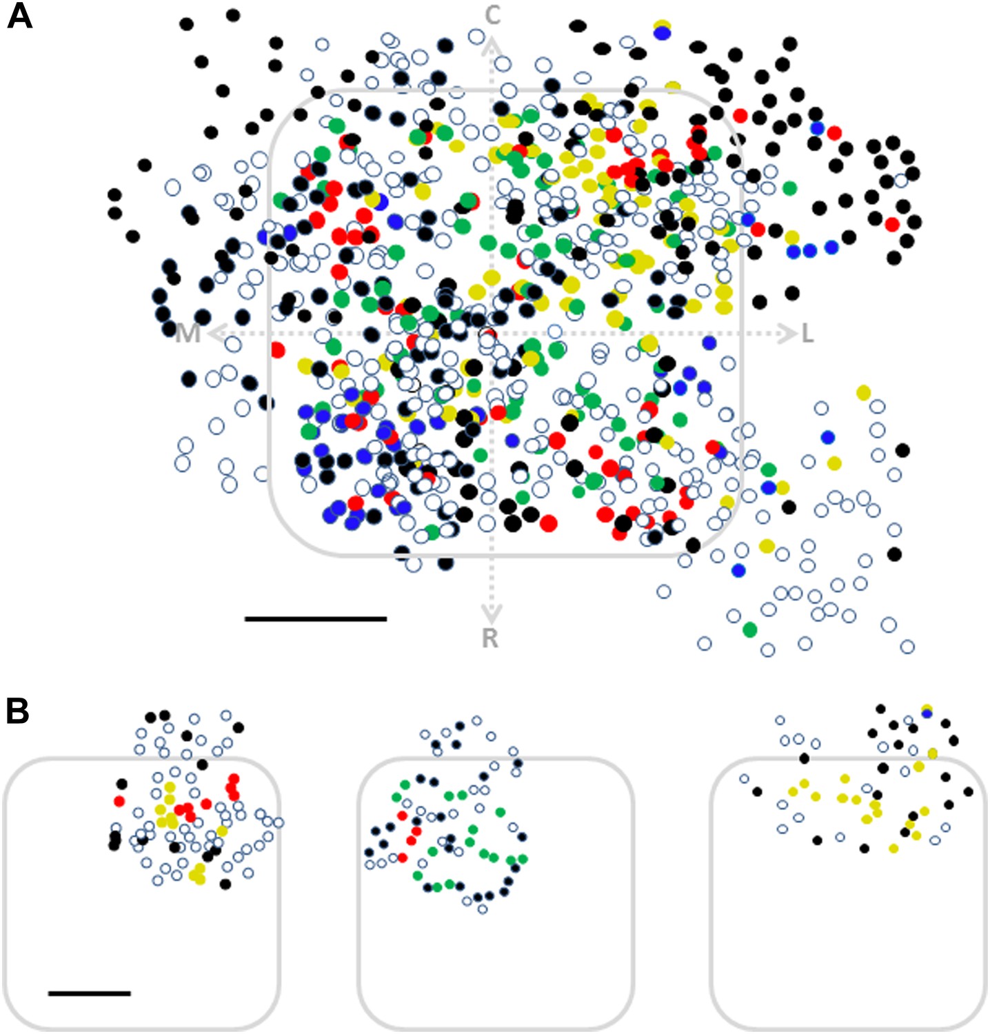
Mapping of texture coarseness, non-selective and non-responsive cells relative to the barrel borders.
(A) Superimposition of the spatial maps of all neurons obtained from 15 experiments onto a ‘normalized’ barrel. These experiments include 12 maps in which cells were predominantly within the barrel boundaries and three additional maps in which neurons were mostly out of the barrel boundaries (blue P120, red P320, green P600, yellow P1000, white non-preferring neurons and black non-responsive neurons) (Scale bar: 100 µm). (B) Three examples of individuals maps showing the non-responding/non-selective cells located in septal regions while selective cells were mostly confined to the barrel (blue P120, red P320, green P600, yellow P1000, white non-preferring neurons and black non-responsive neurons) (Scale bar: 100 µm).
Figure 6—figure supplement 2
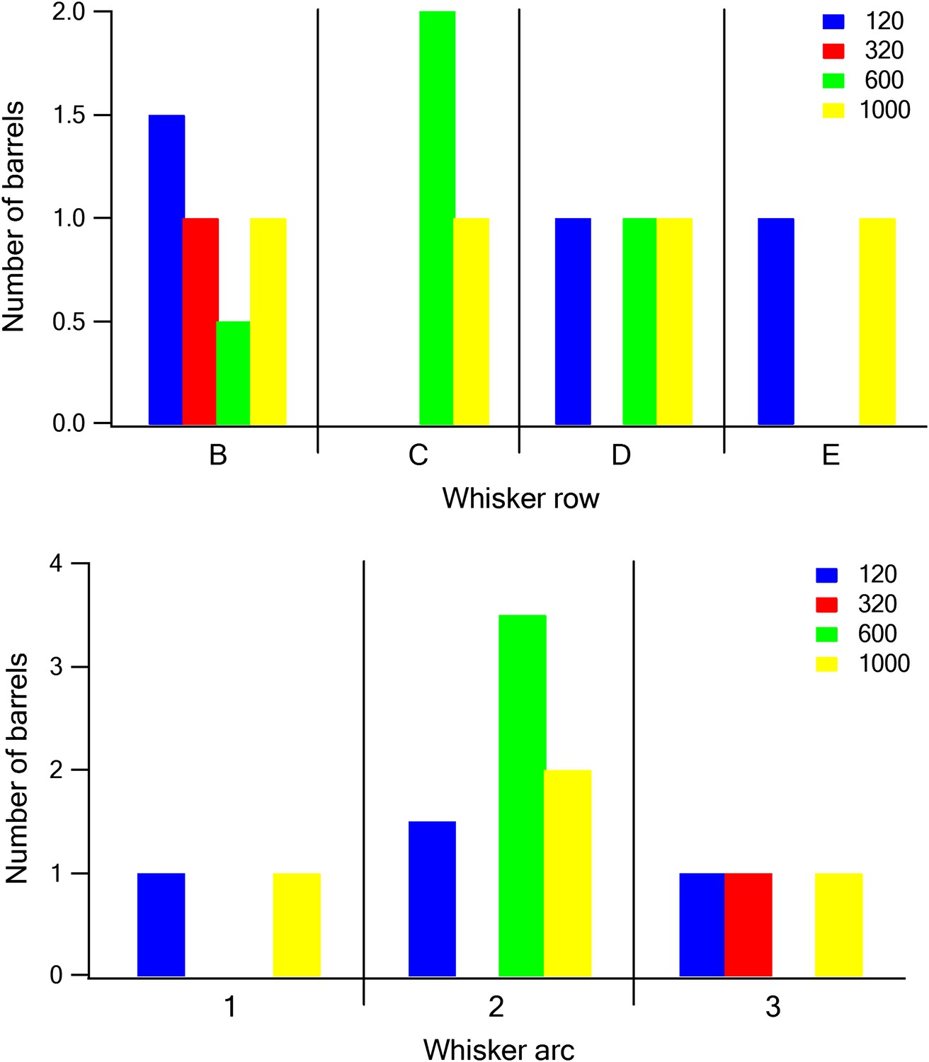
The relationship between barrel location and dominant texture preference.
Each barrel was assigned a dominant texture, which was the texture preferred by the largest number of neurons recorded in the barrel. The number of barrels with the different dominant textures was plotted as a function of the row (upper panel) and arc (lower panel) of the barrel (blue P120, red P320, green P600, and yellow P1000).
Figure 7
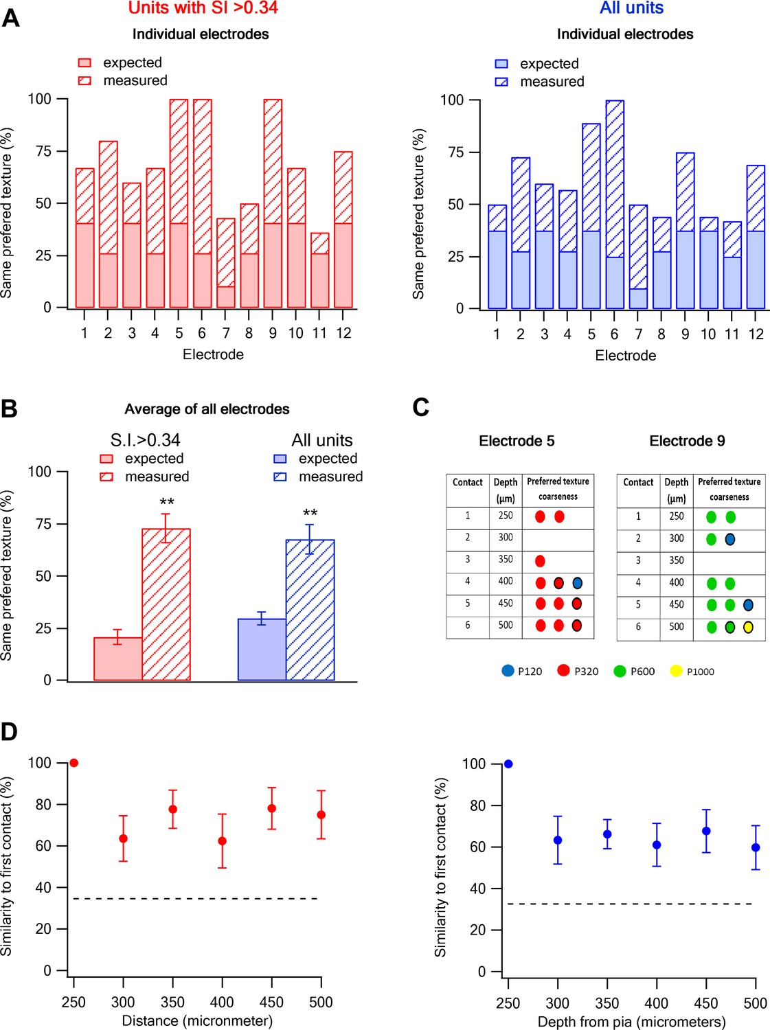
Columnar organization of preferred texture coarseness across layer 2–3 of the barrel cortex.
(A and B) Comparison of the measured (solid) and expected (striped) probabilities for having the same preferred texture coarseness across all neurons recorded in different vertical depth of layer 2–3 using single shaft multi-contact electrodes (inter-contact distance of 50 µm). The data are presented for each individual electrode (A) and for the average of all electrodes (B). The data is also shown for all neurons with S.I. > 0.34 (red) and for all responsive neurons (average ± SEM) (blue). The expected probabilities were calculated from all 133 neurons in 12 electrodes from 12 rats (single multi-contact electrode per rat). (C) The preferred texture coarseness of all units across the six contacts of two example individual single shaft multi-contact electrodes from two different rats (electrode 5 and 9 in panel A) Circle with black perimeter mark units with S.I < 0.35. (D) The probability of retaining the same preferred texture along the different vertical contacts of a single electrode in layer 2–3. We initially determined the dominant preferred texture coarseness in the first contact (250 µm from the pia). Later, we presented the probability neurons will have the same preferred texture coarseness in consecutive contacts. For this analysis, we only used electrodes in which the first recording contact showed a clear dominant preferred texture (at least 66% of neurons with the same preferred texture, 9 out of 12 electrodes with 93 neurons).
Figure 8 with 1 supplement
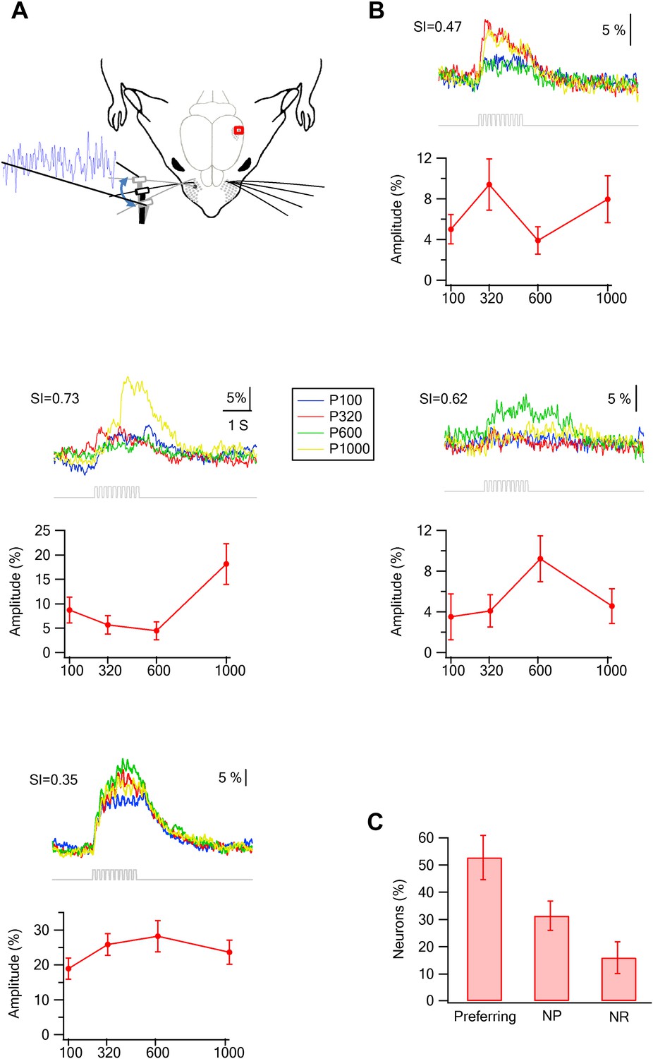
Preferred responses of neurons in layer 2–3 barrel cortex during passive replay of texture-like vibrations.
(A) Experimental set up. The principle whisker was passively stimulated using a galvanometer with four texture-like micro vibrations at amplitudes of 15–30 µm. (B) Examples of the average calcium transient responses (30 repetitions) of four neurons to different passive coarseness-like vibrations simulating the four different textures (upper panels) and their corresponding tuning curves (lower panels; mean ± SEM) as calculated from the peak of the averaged calcium response. For each cell the selectivity index (S.I.) is calculated and presented in the upper left corner (P100-blue, P320-red, P600-green, P1000-yellow). (C) The percentage of neurons (out of 324 neurons in five experiments) that were either texture-like preferring, non-preferring or non-responsive.
Figure 8—figure supplement 1
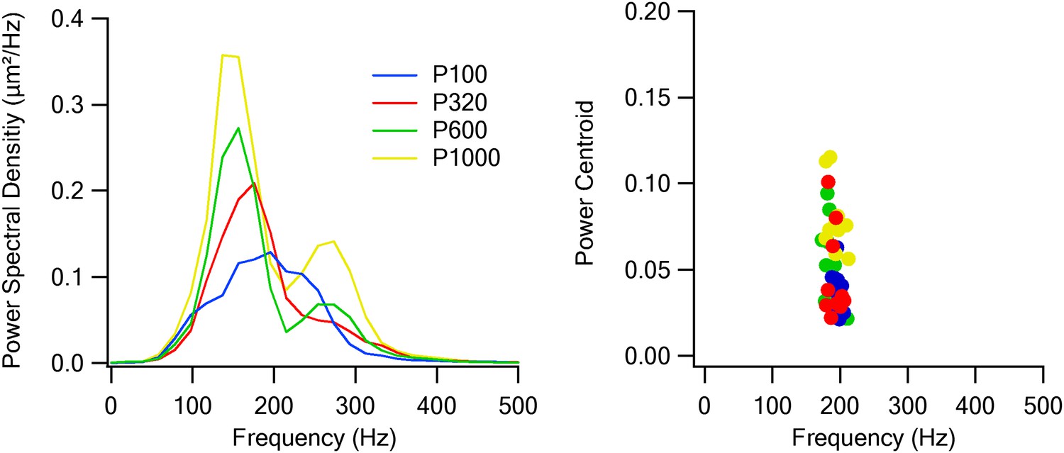
Passive whisker stimulation characteristics.
Power spectral densities (left panel) and power centroids (right panel) of the simulated whisker vibrations of the four textures presented to the whiskers during the experiments using galvanometers.
Figure 9 with 1 supplement
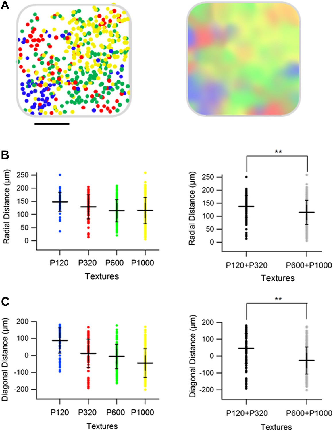
Spatial organization of responding neurons during passive replay of coarseness-like vibrational signals.
(A) (B) Left: texture-like preferring neurons (S.I. ≥ 0.35) from two experiments (upper and lower panels) were color coded according to their preferred simulated coarseness. Right: all responsive neurons (with no S.I. thresholding) were color coded according to their preferred texture coarseness (blue P120, red P320, green P600, yellow P1000, white non-preferring neurons and black non-responsive neurons), and the selectivity strength (S.I. value) which is depicted by the color scale (scale for each color is presented on the right, ranging from 0 to 1). (B) The probability of having 1, 2, 3, or 4 next neighbors with similar preferred simulated coarseness was calculated for the unthresholded maps and compared with the probabilities expected from random spatial distribution for all experiments performed (n = 6 rats) (**p < 0.01). (C) Superimposition of the passive maps from six experiments onto a ‘normalized’ barrel before (left), and after smoothing with a spatial filter (middle panel). In all six maps imaging location was determined using the electroporation method as described in Figure 2. (D) Distance from the MC-LR diagonal (upper) and radial distance from the center of the barrel (lower) of each cell in the different experiments is presented for each texture separately and for the combined coarser textures (black, P120 and P320) and finer textures (gray, P600 and P1000) (**p < 0.01 and *p < 0.05. Comparison of the four textures with ANOVA was not significant for the radial distance and yielded a p < 0.01 for the distance from the MC-LR diagonal.
Figure 9—figure supplement 1
Spatial organization of responding neurons-combined artificial whisking and passive replay of coarseness-like vibrational signals.
(A) Superimposition of maps from all active and passive experiments onto a ‘normalized’ barrel (left panel, scale bar: 100 µm). Right panel shows a smoothened map of the data presented in the left panel. The radial distance from the center of the barrel (B) and distance from the MC-LR diagonal (C) of each cell in the different active and passive experiments is presented for each texture separately (left), and for the combined coarser (black, P120 and P320) and finer textures (gray, P600 and P1000) (right, **p < 0.01). ANOVA testing of the four textures were not significant for the radial distance and significant (p < 0.01) for the distance from the MC-LR diagonal.
Author response image 1

Videos
Video 1
Whisker movement against textures induced by facial nerve stimulation (artificial whisking).
Whisking was induced by facial nerve stimulation (trains of 10 stimuli at 100 Hz repeated at 5.5 Hz). Whisker movement was captured with a fast camera (1000 Hz acquisition rate) while swiping 4 different textures (upper left P1000, upper right P600, lower left P320, lower right P120).
Additional files
Download links
A two-part list of links to download the article, or parts of the article, in various formats.
Downloads (link to download the article as PDF)
Open citations (links to open the citations from this article in various online reference manager services)
Cite this article (links to download the citations from this article in formats compatible with various reference manager tools)
Texture coarseness responsive neurons and their mapping in layer 2–3 of the rat barrel cortex in vivo
eLife 3:e03405.
https://doi.org/10.7554/eLife.03405


