Kinetic competition during the transcription cycle results in stochastic RNA processing
- National Institutes of Health, United States
- National Cancer Institute, National Institutes of Health, United States
- Istituto Italiano di Tecnologia, Italy
Figures
Figure 1 with 2 supplements
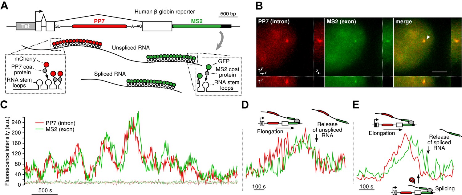
Real-time measurement of transcription and splicing in living cells.
(A) Schematic of the human β-globin report gene construct. Reporter splicing efficiency >95% by qRT-PCR (Figure 1—figure supplement 1C). (B) 3D images of diffraction-limited spot in both channels corresponding to the transcription site (TS, arrow). Bar: 4 µm. (C) Fluorescence fluctuations recorded at the TS reflect stochastic transcriptional events. Dotted lines are background traces recorded in the nucleus, 8 µm away from the TS. (D and E) Examples of pre- and post-release splicing observed when the intron (red signal) disappears simultaneously with (D) or before (E) the exon (green signal).
Figure 1—figure supplement 1

Human β-globin reporter gene.
(A) Detail of the reporter construct (See ‘Materials and methods’). Top schematic drawn to scale. (B) Imaging of gene expression from nascent transcripts (arrow) to protein product (blue channel shows CFP-SKL protein product of the reporter gene accumulating in peroxisomes). Images are maximum intensity projections of z-stacks (Δz = 0.25 μm, exposure = 1 s). (C) Splicing efficiency and (D) poly(A) tail site/length of the β-globin reporter, measured in three conditions: mock-transfected cells and cells transfected with either wild type (WT) or mutant (S34F) splicing factor U2AF1 (see Materials and methods). Error bars are SEM calculated over four measurements. (E) Expected fluorescence time profiles for a single transcript. When the PP7 cassette is transcribed, the red fluorescence signal increases progressively (as RNA stem loops are formed) and plateaus once the polymerase exits the cassette. The same applies to the green fluorescence signal when the PP7 cassette is transcribed. If splicing is post-release, red and green signals drop simultaneously when the unspliced RNA is released and diffuse away. If splicing is pre-release, the red fluorescence drops before the green fluorescence reflecting that intron removal occurred before the release of a spliced transcript.
Figure 1—figure supplement 2
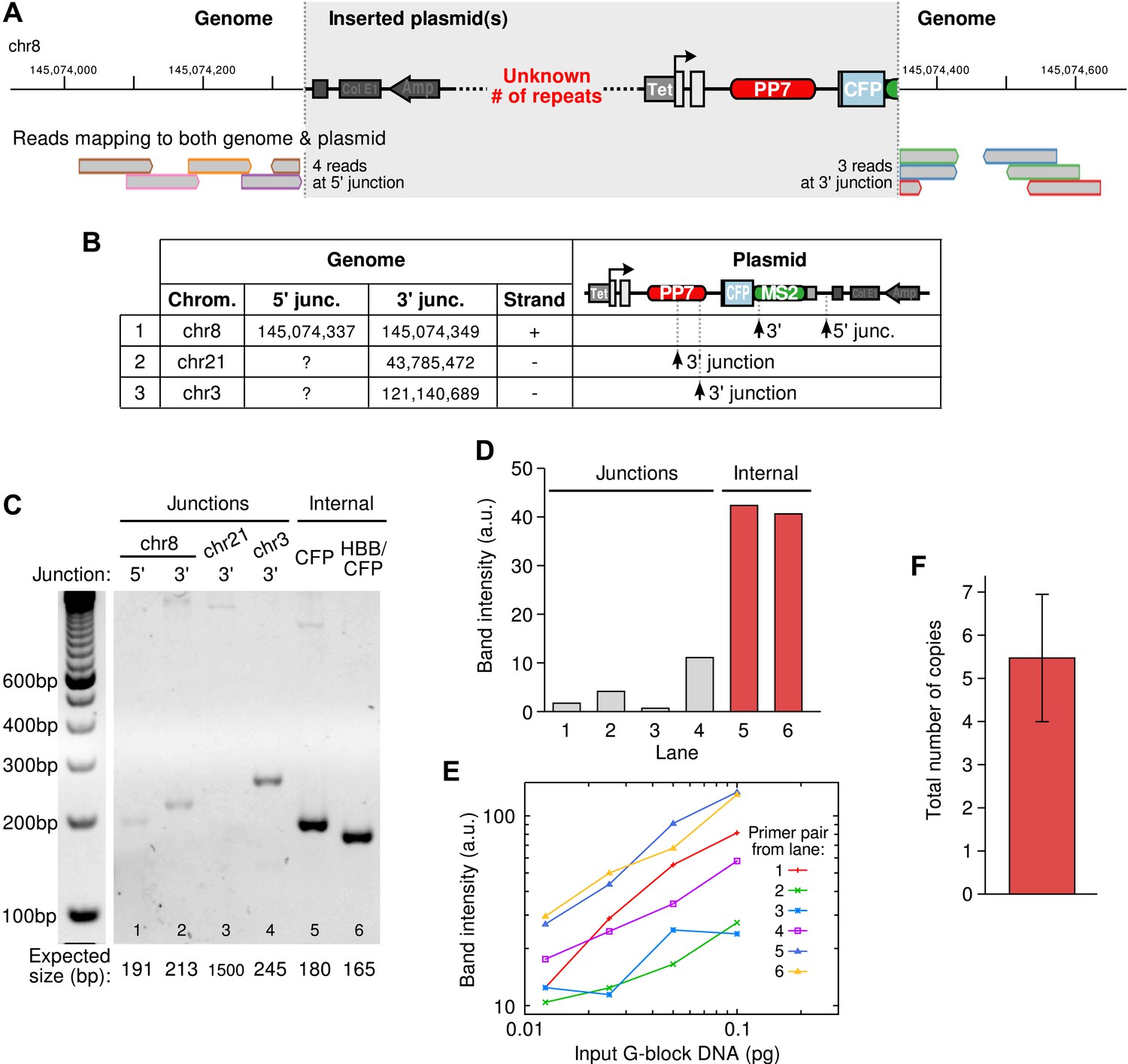
Integration site of the β-globin reporter and copy number analysis.
(A) Example of an integration site of the reporter plasmid as identified by whole genome sequencing. Reads aligning to both genomic and plasmid sequences are shown at the bottom. The alignments identify the genomic position of the insertion and the location of the breaks in the plasmid. The number of repeats of the plasmid at the insertion site cannot be known from sequencing data. (B) Three insertion sites were identified in the cell line. (C) Semi-quantitative PCR was used to confirm the insertion sites and to estimate the total copy number of the integrated plasmid construct in the cell line. (D) Quantification of the PCR products shows, as expected, that amplicons internal to the plasmid were more amplified than the amplicons at the junctions. (E) Calibration curves were made by amplifying varying amounts of G-block DNA carrying the same primer pairs as used in (C). (F) Correcting the data in (D) with the calibration curves in (E) and taking the ratio of internal-to-junction PCR products yields a total copy number of 5.48 ± 1.47. Error is SEM.
Figure 2 with 6 supplements
Transcription and splicing kinetics are revealed by fluctuation analysis of dual-color fluorescence intensity time traces.
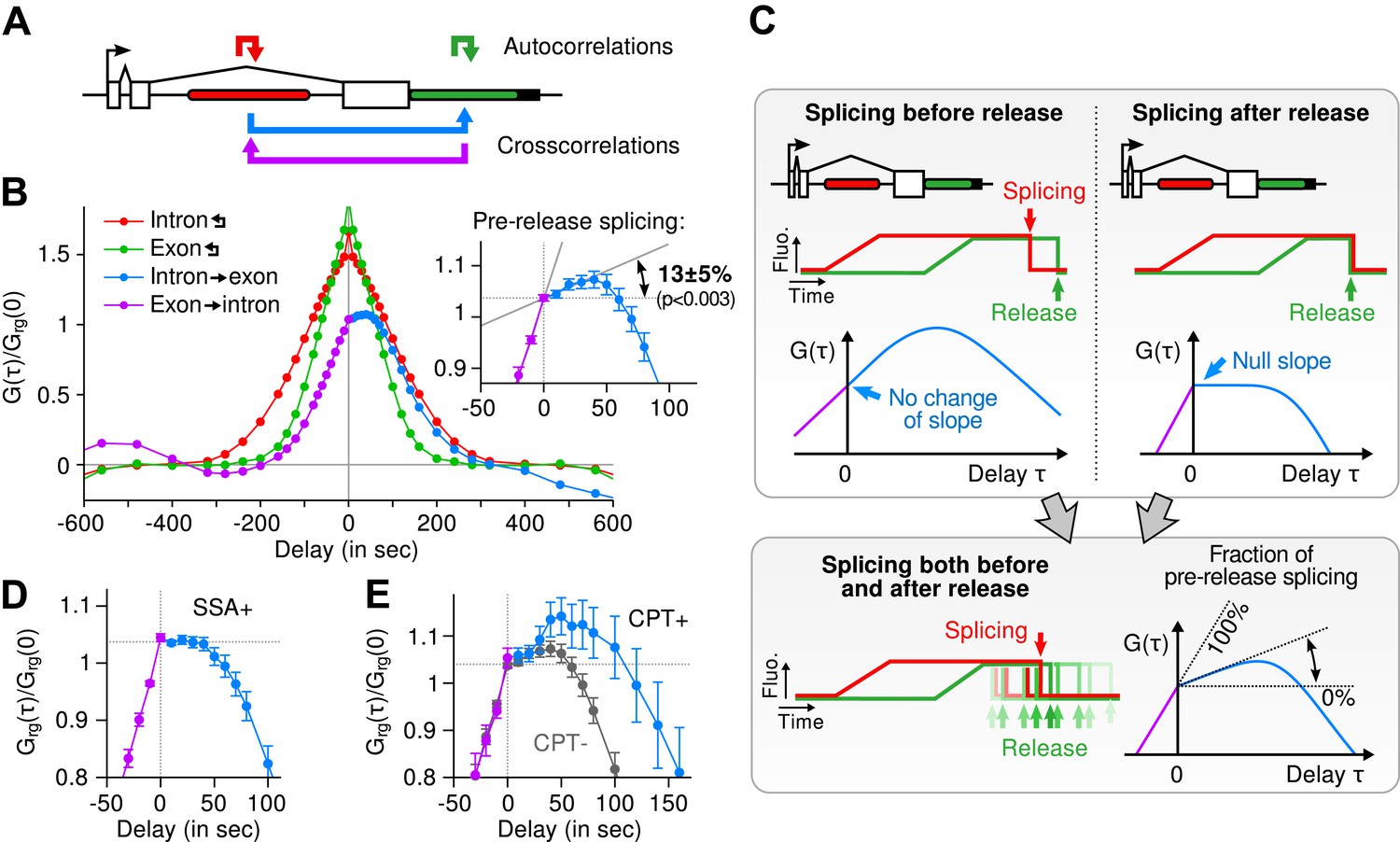
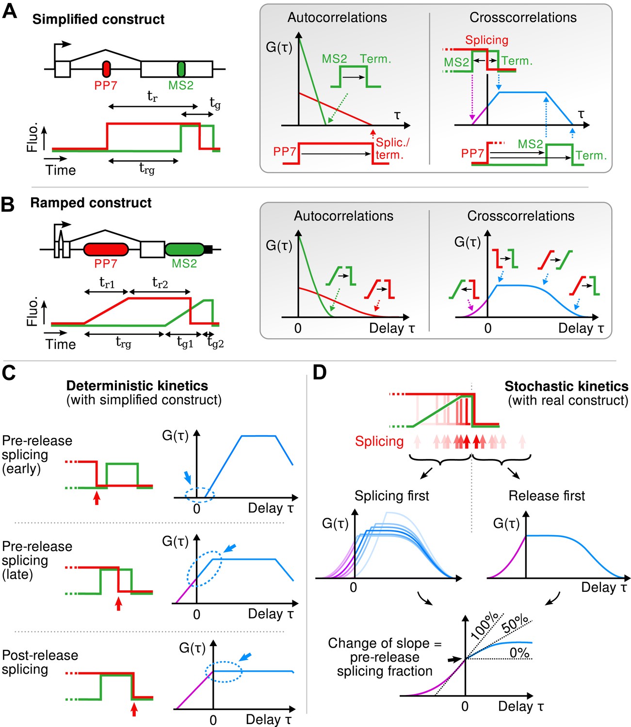
(A) Auto- and cross-correlation functions quantify statistically correlated fluctuations occurring at different time delays, respectively within the same or between two signals. (B) Correlation functions (G(τ)) of experimental time traces (N = 21). Auto-correlations (red and green curves) are symmetrical by construction. Cross-correlations (blue and magenta curves) are two halves of a single continuous curve. Inset: short-delay behavior of the cross-correlation reveals that 13 ± 5% of the RNAs are spliced pre-release (p-value: pre-release fraction ≠ 0% and 100%; z-test). (C) Schematic representing stochastic pre- and post-release splicing. Purely pre-release splicing imposes the cross-correlation to have the same rising slope on both sides of the y-axis, while purely post-release makes the intron-to-exon cross-correlation (blue curve, positive delay) start as a plateau. The change of slope at τ = 0 delay is indicative of the fraction of splicing events occurring before release. (D) Spliceostatin A abolishes pre-release splicing. (E) Camptothecin delays the decay of the intron-to-exon cross-correlation and increases the pre-release fraction. All correlation functions are normalized by the value of the cross-correlation at 0 delay (Grg(0)). Error: SEM (bootstrap). Control correlation functions are shown in Figure 2—figure supplement 1G–H.
Figure 2—figure supplement 1
Fluorescence time traces and correlation functions.
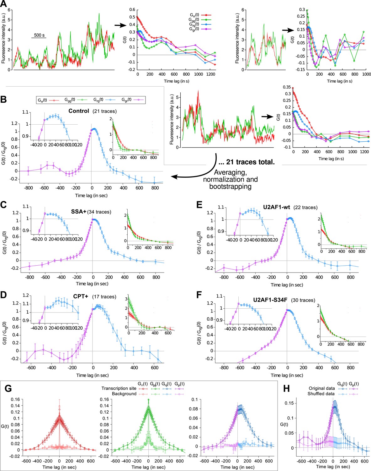
(A) Three examples of dual-color fluorescence time traces recorded at TS (left) and the corresponding correlation functions (right). 21 of such traces were used to compute the average correlation functions shown in (B). (B–F) Correlation functions under different experimental conditions. Each panel shows crosscorrelations (main graph), autocorrelations (right inset) and crosscorrelations magnified around t = 0 (left inset). (G) For each transcription time trace, a background trace was measured in the nucleus at a constant offset from the TS (2.4 μm on average). Correlation functions from these traces reflect technical bias (cell movement, coat protein diffusion, imaging or tracking artifacts) and are mostly flat. (H) Cross-correlation function obtained after swapping the green channels between pairs of time traces (shuffled data) also reveals the absence of technical bias. NB: data in (G) is from a different cell line (same reporter but different genomic insertion site). In all cases except (G and H), all four correlation functions are normalized by Grg(0). Errorbars: SEM (bootstrap).
Figure 2—figure supplement 2
Geometry of the correlation functions.
(A) If fluorescence profiles are approximated by step functions (left), correlation functions are piecewise linear (right). Autocorrelations decrease linearly and reach 0 at a delay equal to the persistence time of the red and green signals. Cross-correlation shows four angles, each reflecting the delay between a rise or fall in the red signal and a rise or fall in the green signal. (B) This can be generalized to the case where fluorescence signals rise as ramps (spanning the width of each cassette). In this case, the sharp angles described above become smooth when one or two of the fluorescence transitions they involve is a ramp. (C) If the red fall precedes the green rise (i.e., splicing precedes transcription of MS2 cassette), crosscorrelation at τ = 0 is null because the two signals never overlap. If the red signal falls while the green signal is up (i.e., splicing occurs after the MS2 cassette but before release), crosscorrelation at τ = 0 is non-null and is increasing with the same slope on either side of the y-axis. Finally, if both signal fall at the same time (i.e., splicing succeeds or coincides with transcript release), the crosscorrelation shows a break of slope at τ = 0, with a positive slope for τ < 0 and a null slope for τ > 0. (D) The correlation functions originating from a heterogeneous (stochastic) population of transcripts is simply the average of the correlation functions for each transcript. Hence, all the pre-release splicing events contribute a positive slope on either site of the y-axis, while all the post-release splicing events only contribute a positive slope on the left side of the axis. The resulting crosscorrelation displays a change of slope that directly reflects the fraction of pre- and post-release splicing events.
Figure 2—figure supplement 3
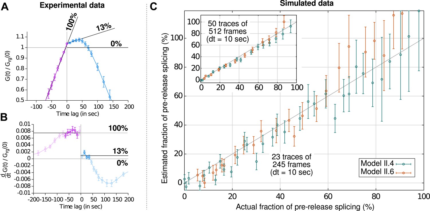
Estimation of the fraction of pre-release splicing from slopes in the crosscorrelations.
In panels (A) and (B), we estimate the fraction of splicing events that occur pre-release from experimental correlation functions (i.e., Figure 2B), by applying the principle shown on Figure 2—figure supplement 2D. Straight lines are fit to the crosscorrelation function on either side of the y-axis (A) by performing a non-linear least-square fit on the derivatives (B). Standard errors are obtained by bootstrapping the derivatives and only the darkened points are used in the fit. The pre-release fraction is obtained as the ratio of the two slopes. (C) Simulated data (from models II.4 and II.6; see ‘Materials and methods’ and Supplementary file 2) were used to assess the accuracy of this method. The pre-release fraction effectively observed in the simulations is compared to the one obtained by fitting the slopes of the correlations functions. Each point corresponds to a set of simulations preformed with a given set of parameters. The amount of data used per point in the main graph is similar to the experimental data shown in (A) and is higher in the inset, yielding a more precise estimation.
Figure 2—figure supplement 4

Mechanistic schemes.
This figure presents the five mechanistic schemes that are compared to our data. The central part of each panel depicts the fluorescence time profiles lined up with the reporter construct, indicating the names of the time distributions of the different sections of the profile (i.e., time the polymerase spends in each region of the construct). The right part of each panel indicates what is assumed in terms of kinetic relationship between splicing (i.e., intron removal), elongation (i.e., progression or pausing), and release (i.e., including some 3′ end processing time or retention on the chromatin). (Scheme I) Splicing never happens pre-release. (Scheme II) Once the 3′ splice site (3′ss) is reached and as long as the RNA is as the transcription site, splicing is kinetically independent from all other processes such as elongation and 3′ end processing/retention. It means that affecting either process will change the balance of post- vs pre-release splicing. (Scheme III) Once the 3′ splice site is reached, an obligatory checkpoint forces the polymerase to pause until the splicing reaction completes. (Scheme IV) The transcript can only be spliced once the 3′ end of the gene is reached. Once the intron is removed, the RNA may be released after an additional processing/retention time. (Scheme V) Splicing may happen any time after the 3′ss is reached but a checkpoint mechanism ensures the RNA is spliced before its release.
Figure 2—figure supplement 5
Model comparison using a Bayesian Information Criterion (BIC).
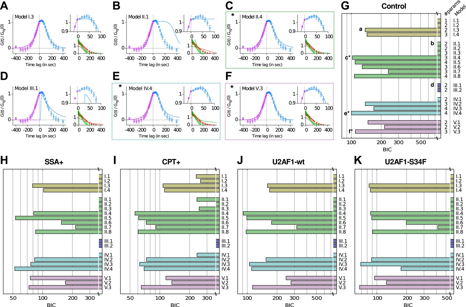
(A–F) Examples of best fits (lines) onto experimental correlation functions (circles; untreated, untransfected condition) with 6 of the 21 competing models. Left and top right graphs: crosscorrelations; bottom right graph: autocorrelations. (G–K) All 21 models were compared on five experimental conditions, using the BIC score (the lower the better, see Supplementary file 1—Appendix 3). The number of parameters for each model is indicated on the right of panel (G). The BIC accounts for the variable number of parameters. * Models II.4, IV.4, and V.3 are the three models that we retain from our analysis.
Figure 2—figure supplement 6
Counting transcripts at the transcription site.
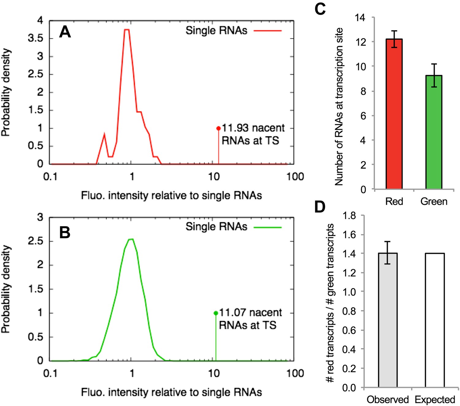
(A–B) The average intensity of the single-RNA particle diffusing in the nucleus detected in one channel of a confocal video (e.g., Figure 4A or Video 5) was used to normalize the intensities of all the spots found in that channel. Panels (A) and (B) show the distribution of normalized intensities of all the single RNAs (centered around 1) as well as the transcription site (TS) for the red and the green channels respectively. This allows estimating the average number of RNAs at the TS that are labeled in red and green. (C) Repeating this analysis for multiple cells (N = 9) and averaging shows that there are more red RNAs than green RNAs. (D) The average of the ratio between the number of red and green RNAs at the TS is very close to the expected value of 1.4 calculated from the fitting parameters shown in Table 1. Errors: SEM over cells.
Figure 3 with 1 supplement
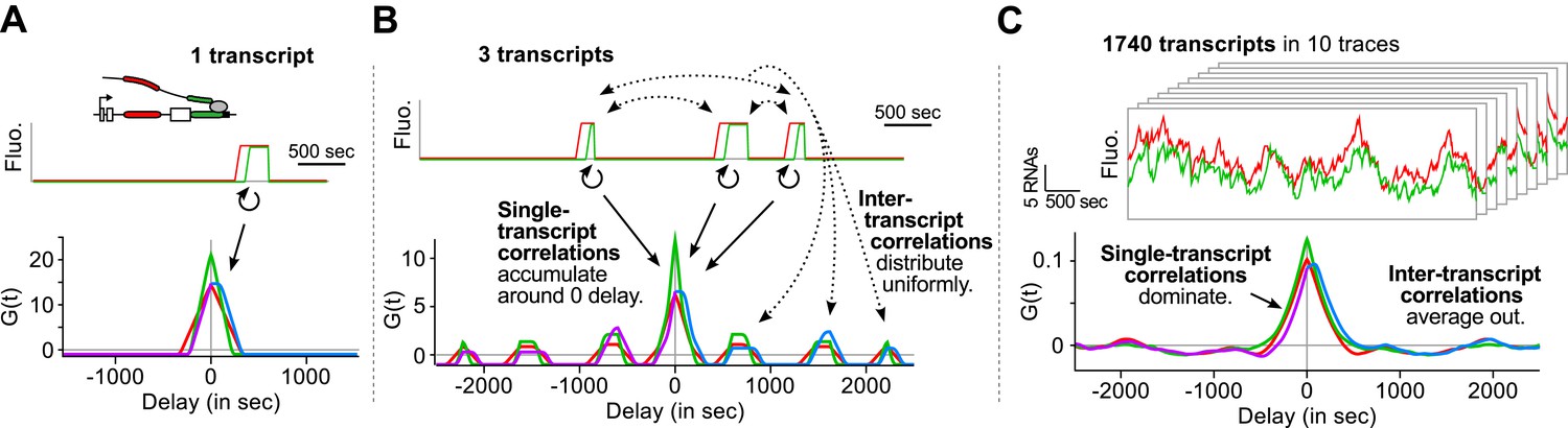
Correlation functions reflect single-transcript kinetics.
(A) A dual-color time trace with a single transcription event yields correlation functions with features around 0 delay and flat elsewhere. (B) When several transcription events are present in a time trace, the correlation coming from each individual RNA accumulates around 0 delay, while all the correlation between pairs of RNAs distributes uniformly on the delay axis. (C) When there are many transcription events per time trace and/or many traces are used to produce an average correlation function, the correlation from single transcripts dominates and that from pairs of transcripts averages out. The resulting correlation functions hence reflect single-transcript kinetics. Time traces shown are simulations where the statistics of transcript kinetics are similar to those we measured by live cell imaging. Traces in (C) have the same duration and number of transcripts as estimated in experimental data (e.g., Figure 1C). See Video 4 for an animation of how the correlation functions converge as the number of transcripts increases.
Figure 3—figure supplement 1
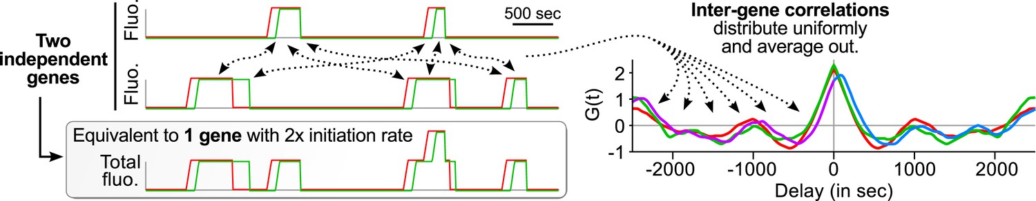
Correlation functions with several gene copies at the TS reflect single-transcript kinetics.
The same principles as shown on Figure 3 can be applied to a case where several independent genes are at the transcription site (TS). The contributions of pairs of transcripts from distinct genes (inter-gene) behave like inter-transcript correlations in Figure 3B and hence distribute uniformly on the delay axis and simply average out.
Figure 4 with 2 supplements
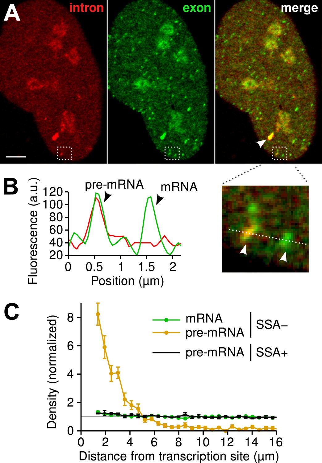
Visualization of splicing occurring after release from chromatin.
(A) Individual frames from live-cell confocal imaging showing intron (red dots), exon (green dots), and the merged image. White arrow: TS. Bar: 4 µm. (B) Fluorescence intensity profile along the line in the inset shows co-localized intron/exon (unspliced pre-mRNA) and exon only (spliced mRNA). (C) Radial distributions of mRNA (green) and pre-mRNA (orange), as well as pre-mRNA under SSA treatment (black) are shown as a function of distance from the TS. Density distributions are normalized by the distribution of random (uniform) positions within the nucleus (see ‘Materials and methods’). Error: SEM (bootstrap over 9 cells).
Figure 4—figure supplement 1
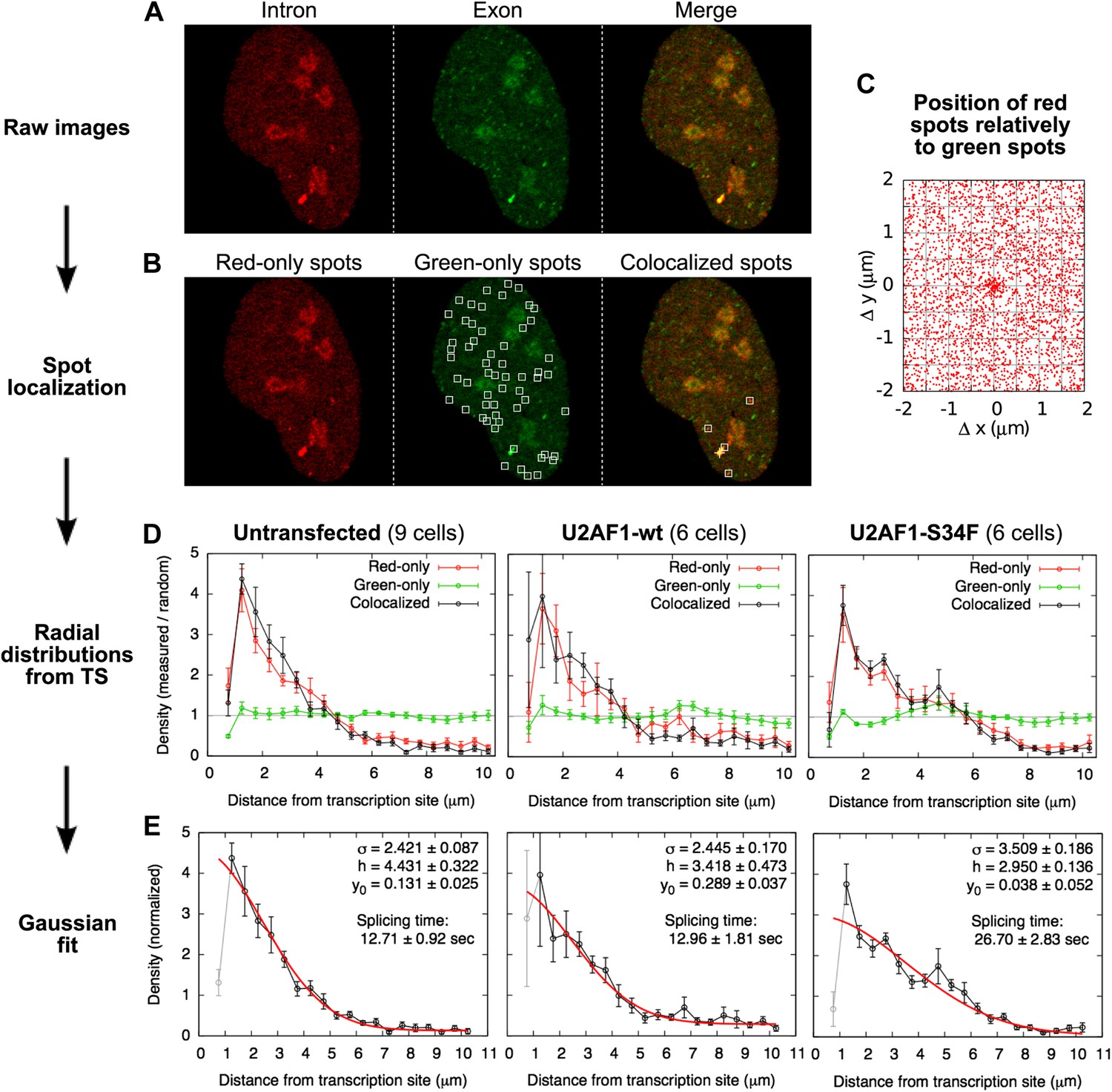
Localization of single RNAs diffusing in the nucleus.
(A) Example of a raw confocal image from Video 5. Many particles are visible in the exon channel (center). The intron channel (left) shows fewer particles that colocalize with green ones (See merge, right). (B) The spot-finding algorithm, run independently on the red and green images, generates a list of red and green spot coordinates. Spots colocalized by less than 250 nm were paired, yielding a list of red-only, green-only, and colocalized particles. (No spots are indicated on the red image since all of the red spots colocalize with a green one in this frame.) (C) Plotting, for all the frames, the position of all the red spots relative to all the green spots in the same frame reveal a population of particles colocalizing in the two channels within a 250-nm radius. (D) The radial distribution of the distances between colocalized particles and the transcription site is shown here normalized by the radial distribution of random locations within the nucleus. Three exprimental conditions are shown: for three experimental conditions: untransfected cells and cells transfected with wild-type (wt) or mutant (S34F) U2AF1. The depletion at very short distances is a technical artifact of spot detection (2 very close particles are detected as a single one). (E) These distributions are fitted with a Gaussian function with three parameters: standard deviation σ, height h, and baseline y0. Errors: SEM over cells.
Figure 4—figure supplement 2

Measure of RNA diffusion in the nucleus by RICS.
(A) Spatial RICS autocorrelation function of green channel from a RICS measurement. Color code is the same as the vertical axis of (B). (B) A 2D fit to a two component diffusion model gives a good fit with fast and slow moving components (60%, 1.64 μm2/s and 40%, 0.095 μm2/s). Bottom graph is the fit and top graph is the residual. (C) Resulting measurements of free coat protein (MS2-GFP) and mRNA diffusion coefficients. Error bars: SEM.
Figure 5
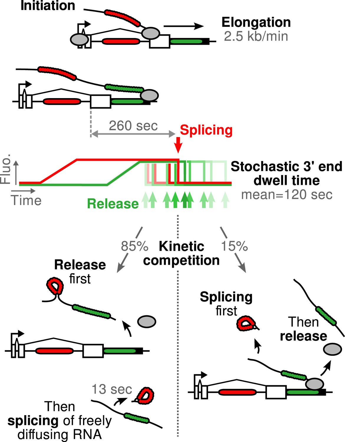
Schematic of β-globin transcription cycle kinetics.
Transcript synthesis and processing can occur through different pathways, the choice of which is governed by a kinetic competition between transcription and splicing. After transcription of the 3′ splice site, intron removal takes about 260 s and elongation until the end of the gene, about 55 s. Hence, splicing does not occur during elongation. The transcript is retained at the 3′end of the gene for a stochastic amount of time that can be shorter or longer than the remaining time to excise the intron. This results in two possible outcomes: either an unspliced pre-mRNA is released and then spliced very rapidly or splicing occurs while the transcript is retained on chromatin before being released.
Figure 6

The U2AF1-S34F mutant acts as a dominant negative by delaying splicing to post-release.
(A) Expression of U2AF1-cerulean does not alter pre-release splicing compared to the un-transfected control. Expression of U2AF1-S34F-cerulean abolishes splicing at the TS (horizontal slope of the intron-to-exon cross-correlation, blue curve). (B) Pre-mRNA (red, marked by squares) are enriched around the TS (arrows) indicating that splicing still occurs faster than diffusion. The enrichment is broader in the presence of U2AF1-S34F despite the similar spatial distributions of both proteins. (C) Gaussian fits onto pre-mRNA radial distance distributions from the TS. (D) The U2AF1-S34F mutant defers splicing to occur entirely away from the TS (fractions obtained from model fits in Table 1) and increases post-release splicing time. ** p < 0.005 (two-sided z-test vs untransfected control). (E) Two-color single-molecule FISH on endogenous FXR1 transcripts. Unspliced pre-mRNA (co-localization of intronic and exonic probe) appears in the vicinity of TSs (the 4 bright dual-color spots). (F) The fraction of pre-mRNA transcripts in the nucleus in the presence of wt or mutant U2AF1. (G) Spatial distribution of pre-mRNAs near TSs in the presence of wt or mutant U2AF1 (N > 400 cells). Radial distributions show density of pre-mRNA normalized by density of mRNA. Bars: 4 µm. Error: SEM over cells (bootstrap).
Videos
Video 1
Time-fluctuating transcription sites.
Cells show a diffraction-limited fluorescent spot colocalizing in both colors (red: intron, green: exon), corresponding to the transcription site of the reporter gene. The fluorescence intensity of each site fluctuates over time as nascent transcripts are synthesized, spliced, and released from the transcription site. Large orange shapes in nuclei are nucleoli (Ferguson and Larson, 2013).
Video 2
Tracking of a transcription site in 4D.
The video shows, for the intron and exon signals (left and center panels), the maximum intensity projected image from the top (square image) and from the sides (rectangle images), revealing the transcription site (TS) in three dimensions (3D) and over time (4D). Image analysis is used to track the TS over time in both colors. The blue box and cross indicate the location of the TS as found by the tracking algorithm. The right panel is the merge of both signals.
Video 3
Spliced RNAs diffusing in the nucleus and the cytoplasm.
Cells are imaged here with a high laser power and a short exposure time so that diffusion of single RNAs can be appreciated. It reveals a population of transcripts diffusing in both the nucleus and the cytoplasm, as evidenced by fast fluctuations observed in the exon signal (right panel). These transcripts are, for the most part, already spliced since the intron signal (center panel) does not show the same fluctuations. In these imaging conditions, unspliced transcripts are only visible at the transcription site (bright spot in the nucleus colocalizing in both color; see merge in left panel).
Video 4
Correlation functions reveal single transcript kinetics.
This video shows the convergence of the correlation functions for increasing number of transcripts in a time trace. See also Figure 3.
Video 5
Single-RNA imaging reveals a transient population of unspliced transcript diffusing away from the transcription site.
Using high-power confocal laser scanning microscopy, we were able to observe single transcripts with a better temporal resolution than with widefield imaging (Video 3). The video shows a single cell with an active transcription site (TS, bright spot visible in both signals) and diffusing RNA particles (left: intron, center: exon, right: merge). Although most of the RNAs diffusing in the nucleus are spliced (visible only in the exon signal), few unspliced RNAs (visible in both colors) are detectable in the vicinity of the TS as they diffuse away. Spatial distribution and diffusion analyses revealed that this population is very transient (Figure 4C and Figure 4—figure supplements 1 and 2). Large shapes in the nucleus are nucleoli (Ferguson and Larson, 2013).
Video 6
Single-RNA imaging with splicing inhibitor SSA.
Imaging conditions are identical as in Video 5, but cells are treated with splicing inhibitor spliceostatin A (SSA). RNAs diffusing in the nucleus are now visible in both color, indicating that they are unspliced.
Video 7
Spatial distribution of pre-mRNA with wild type or mutant U2AF1.
Left and right images show a cell that was transfected with the wild type (wt) or the mutant (S34F) version of splicing factor U2AF1. Both the image show the intron channel. The enrichment of unspliced pre-mRNA (red spots) diffusing in the vicinity of the transcription site is broader in the case of the mutant, showing that splicing rate is slower. Imaging conditions are identical as in Video 5.
Tables
Table 1
Kinetics of transcription and splicing under different experimental conditions
| Elongation rate (kb/min) | Mean 3' end dwell time (sec) | Splicing time (sec) | Pre-release fraction (%) | |
|---|---|---|---|---|
| Control | 2.60 ± 0.16 | 116.1 ± 5.8 | 267 ± 9 | 15.9 ± 3.2 |
| SSA+ | 2.41 ± 0.26 | 126.7 ± 5.7 | 485 ± 62 ** | 3.5 ± 2.4 ** |
| CPT+ | 1.44 ± 0.09 ** | 111.0 ± 10.3 | 251 ± 10 | 24.9 ± 6.9 |
| U2AF1 (wt) | 2.24 ± 0.27 | 120.7 ± 4.9 | 280 ± 8 | 16.6 ± 3.3 |
| U2AF1-S34F | 2.64 ± 0.11 | 166.0 ± 7.0 ** | 694 ± 176 * | 2.1 ± 2.6 ** |
-
The table shows result of fits with model II.4 (‘Materials and methods’ and Supplementary file 2). Pre-release fraction is deduced from the 3 other parameters. Errors are propagated SEM from correlation functions. * p-value<0.05, ** p-value<0.005 (two-sided z-test vs control).
Additional files
-
Supplementary file 1
Mathematical analysis of the correlation functions.
- https://doi.org/10.7554/eLife.03939.028
-
Supplementary file 2
Models from mechanistic schemes. From each scheme depicted in Figure 2—figure supplement 4, we derive a series of models by simply affecting the arbitrary distributions A(t), B(t), C(t), … to specific ones (columns Time distributions). Each model represents a specific mechanism (column Description) and involves a different number of parameters (column Params). Some models may be excluded simply because, by construction, they cannot reproduce certain basic geometric properties of the crosscorrelation functions (columns Features of Grg(0); properties described in Figure 2—figure supplement 2C), or because they do not allow for unspliced transcripts to be released (last column), as observed experimentally (Figure 4, Figure 4—figure supplement 1 and Video 5). 3′ss: 3′ splice site.
- https://doi.org/10.7554/eLife.03939.029
-
Source code 1
Source code and executable file for the spot tracking software.
- https://doi.org/10.7554/eLife.03939.032
Download links
A two-part list of links to download the article, or parts of the article, in various formats.
Downloads (link to download the article as PDF)
Open citations (links to open the citations from this article in various online reference manager services)
Cite this article (links to download the citations from this article in formats compatible with various reference manager tools)
Kinetic competition during the transcription cycle results in stochastic RNA processing
eLife 3:e03939.
https://doi.org/10.7554/eLife.03939


