Automatic discovery of cell types and microcircuitry from neural connectomics
- University of California, Berkeley, United States
- Northwestern University, United States
- Rehabilitation Institute of Chicago, United States
Figures
Figure 1
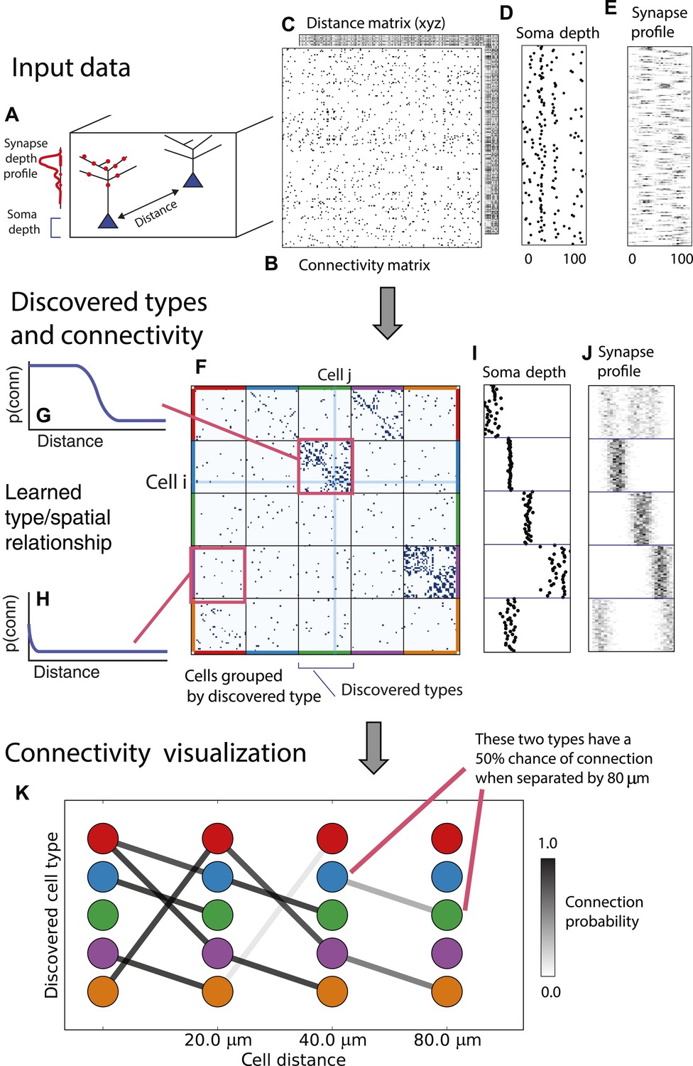
Deriving circuitry and cell types from connectomics data.
(A) As input we take the connectivity between cells (B), the distance between them (C), the depth of the cell bodies (D), and the depth profile of the synapses (E). (F) Our algorithm discovers hidden cell types in this connectivity data by assuming all cells of a type share a distance-dependent connectivity profile, similar depth, and a similar synaptic density profile, with cells of other types. This results in a clustering of the cells by those hidden types. (F) Shows the cell connectivity matrix with cells of the same type grouped together. (G) Shows the learned probability of connection (p(conn)) between our different types at various distances—in this case, the cells are likely to connect when they are close. (H) Shows the probability of connection (p(conn)) between two cell types that very rarely connect—there is a background ‘base’ connection rate to account for errors in data, but the probability is very low. (I) Shows that we also recover the expected laminarity of types and the depth-specific (J) synaptic connectivity. (K) We then plot how the connectivity between these types changes as a function of distance between the cell bodies to better understand short-range and long-range connectivity patterns.
Figure 2
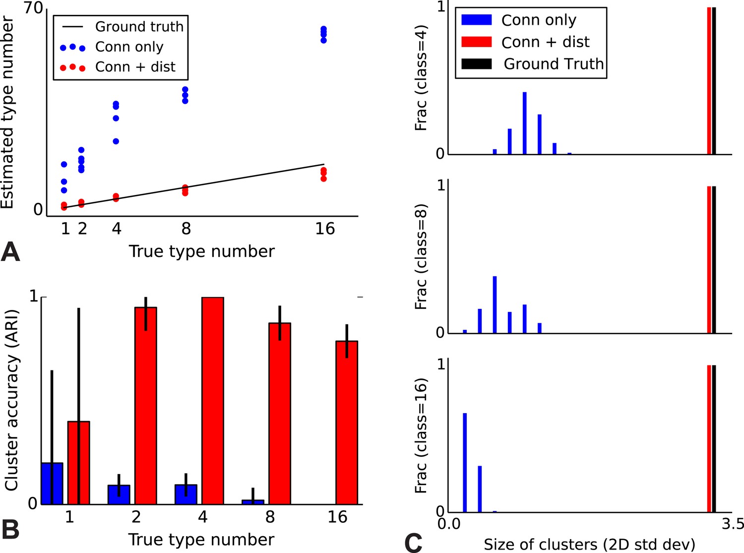
Correct recovery of true numbers of hidden types in synthetic data when incorporating spatial information.
(A) The infinite stochastic block model (which only uses connectivity information) over-estimates the number of classes as it fails to take distance into account, whereas our modeling of the combination of distance and connectivity finds close to the true number of classes. Conn: connectivity; dist: distance. (B) As we increase the true number of types, our method continues to find the correct clustering (as measured by the adjusted Rand index, ARI) whereas the infinite stochastic block model (iSBM) overclusters and thus poorly matches ground truth. (C) We examine the spatial extent (size) of the discovered types (clusters) by measuring the two-dimensional standard deviation of the cell locations. The y-axis indicates what fraction of the discovered types had a given spatial extent. Without incorporating distance, we identify a large number of small, spatially-localized types. With distance, we see a correct recovery of the spatial extent of each type.
Figure 3
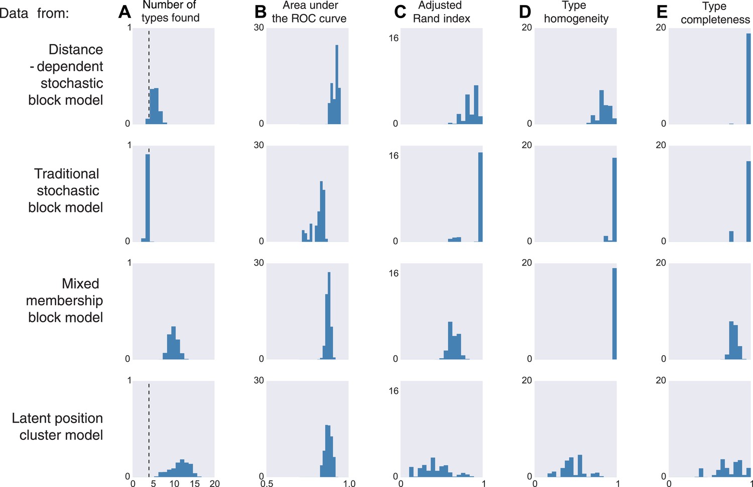
Model inferences when the true generating model differs from our distance-block-model prior.
Horizontal columns show results with synthetic data generated according to the distance-dependent stochastic block model, the non-distance-dependent stochastic block model, the mixed membership block model, and the latent position cluster model. In all cases histograms represent posterior distribution over the indicated metric. (A) The number of types found by the model; the vertical dashed line indicates the ‘true’ type number (not applicable to the mixed membership model). (B) The area under the receiver operating characteristic (ROC) curve, indicating link prediction accuracy. (C, D, E) Clustering metrics quantifying degree of type agreement with known ground truth.
Figure 4
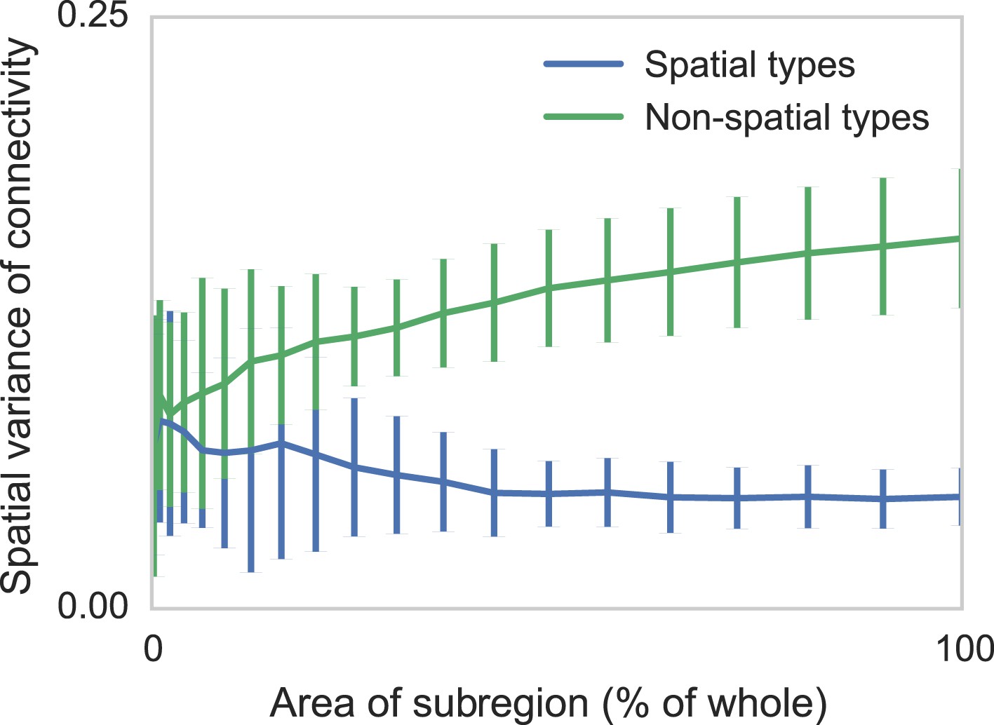
Two sets of generated synthetic data, one with spatially dependent connectivity and one without.
We measure the variance in the connectivity-distance plot for randomly selected regions of each dataset, ranging from single cells to the entire volume. We see that while selecting too small a region can destroy the appearance of distance-dependent connectivity, it does not create it in non-spatial data.
Figure 5
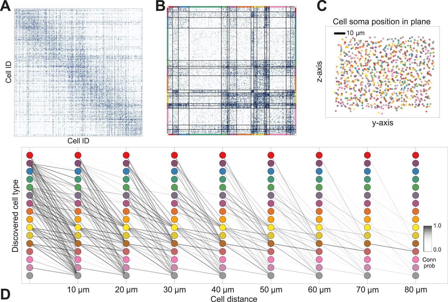
Discovering cell classes in the mouse retina connectome.
Here we show the maximum a posteriori (MAP) estimate for the types in the mouse retina data. (A) Input connectivity data for 950 cells for which soma positions were known. (B) Clustered connectivity matrix; each arbitrary color corresponds to a single type and will be used to identify that type in the remainder of the plot. (C) The spatial distribution of our cell types—each cell type tessellates space. Colors correspond to those in (B). (D) Connectivity between our clusters as a function of distance—the cluster consisting primarily of retinal ganglion cells (brown nodes on the graph) exhibits the expected near and far connectivity. Conn prob: probability of connection.
Figure 6
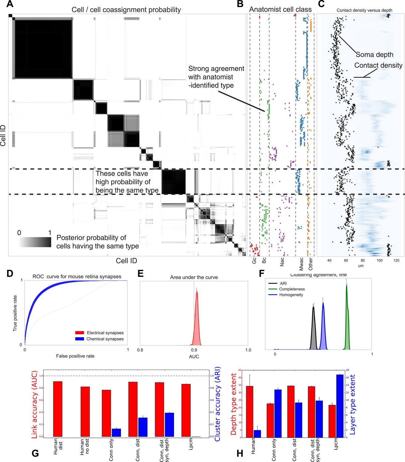
Visualizing type inference uncertainty.
Our fully Bayesian model gives a confidence estimate (posterior probability) that any two given cells are of the same type. In (A) we visualize that cell–cell coassignment matrix, showing the probability that cell i is of the same type as cell j on a range from 0.0 to 1.0. The block structure shows subsets of cells which are believed to all belong to the same type. For comparison, (B) shows the anatomist-defined type for each cell, grouped broadly into the coarse types identified in the previous panel. (C) Link versus cluster accuracy. (D) The posterior distribution of receiver operating characteristic (ROC) curves from 10-fold cross-validation when predicting connectivity, as well as (E) the area under the curve (AUC) and (F) the type agreements with known neuroanatomist types. ARI: adjusted Rand index. Model comparison, showing using human-discovered types with and without distance information, as well as our model incorporating just connectivity, connectivity and distance, or connectivity, distance, and synaptic depth (as well as the alternative latent position cluster model, see text). (G) A comparison of the predictive accuracy (AUC) for hand-labeled anatomical data, versus inclusion of additional sources of information, as well as the clustering accuracy. Note that our model sacrifices very little predictive accuracy for additional clustering accuracy. By comparison, conventional methods fail at one or both. ARI: adjusted Rand index. (H) The spatial extent (in depth and area) of the types identified by humans and our various algorithmic approaches.
Figure 7
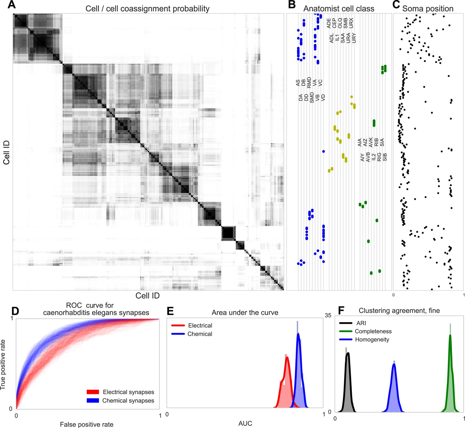
Discovering connectivity and type in C. elegans.
(A) Posterior distribution on cell connectivity as a function of discovered type, similar to Figure 6. In (B) we plot neuroanatomist-derived types along with their labels. Our model shows a high probability of motor neurons, sensory neurons, and various interneuron classes being of the same type. Soma positions along the body axis are plotted in (C) where we see that we cluster spatially distributed motor neurons together, whereas head sensory neurons are more likely to be grouped together as well. (D) The receiver operating characteristic (ROC) curves for held-out link probability for both the electrical synapses (gap junctions) and chemical synapses in C. elegans. (E) The posterior distribution of the area under the ROC curve (AUC) for the curves in (D). (F) Measurements of the agreement of our identified cell types compared to neuroanatomists. The high completeness but low homogeneity (and corresponding low adjusted Rand index, ARI) reflects our model's tendency to group multiple types into a single type.
Figure 8
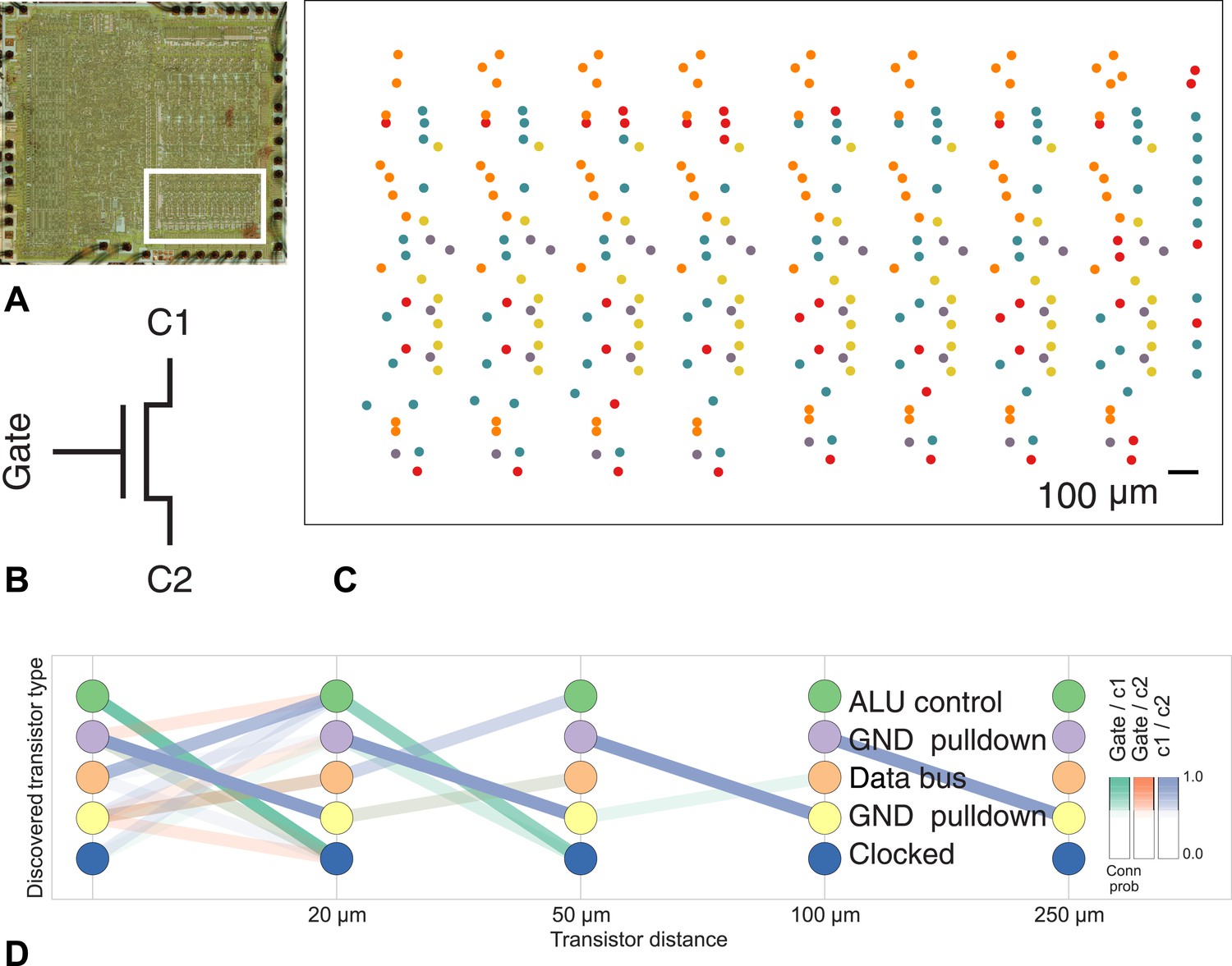
Discovering connectivity and type in the MOS 6502 microprocessor.
(A) The micrograph of the original microprocessor, with the region containing the registers under study highlighted. (B) Our graph consists of the interconnections of MOS field-effect transistors with three terminals, Gate, C1, and C2. The reconstruction technique did not permit resolution of C1 and C2 into source and drain. (C) The spatial distribution of the transistors in each cluster show a clear pattern. (D) The clusters and connectivity versus distance for connections between Gate and C1, Gate and C2, and C1 and C2 terminals on a transistor. Purple and yellow types have a terminal pulled down to ground and mostly function as inverters. The blue types are clocked, stateful transistors, green control the ALU and orange control the special data bus (SDB).
Figure 9
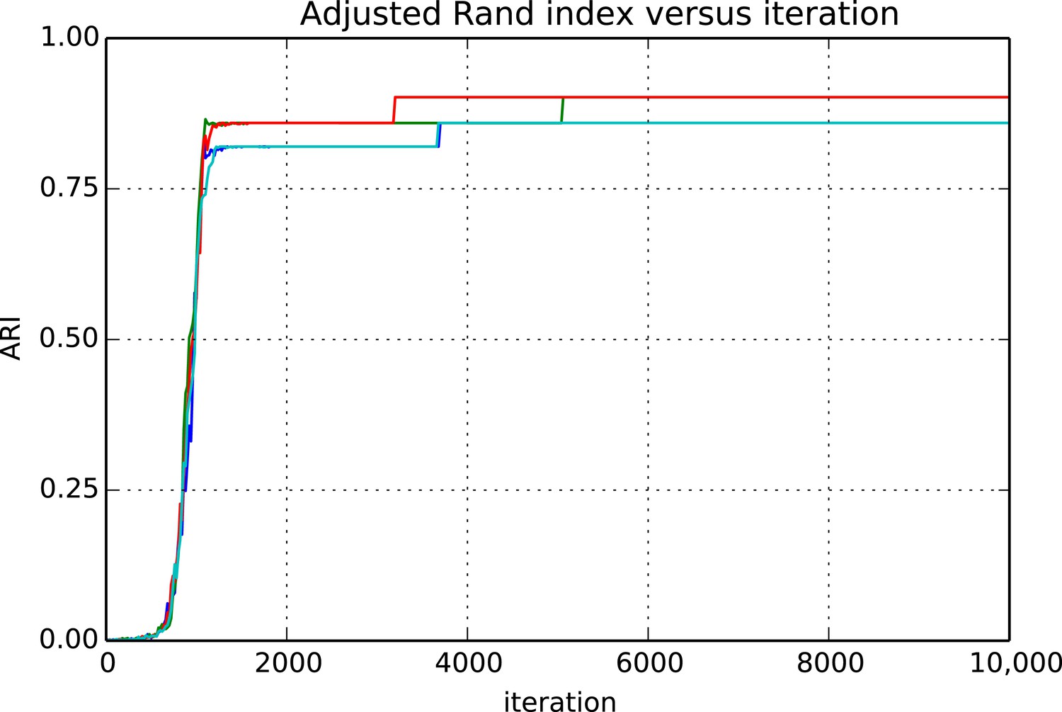
Adjusted Rand index (ARI) for synthetic data as a function of run iteration.
https://doi.org/10.7554/eLife.04250.011
Figure 10
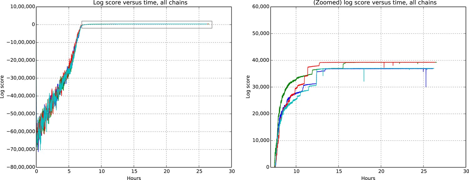
Total model score (log score) versus wall clock time.
https://doi.org/10.7554/eLife.04250.012
Figure 11
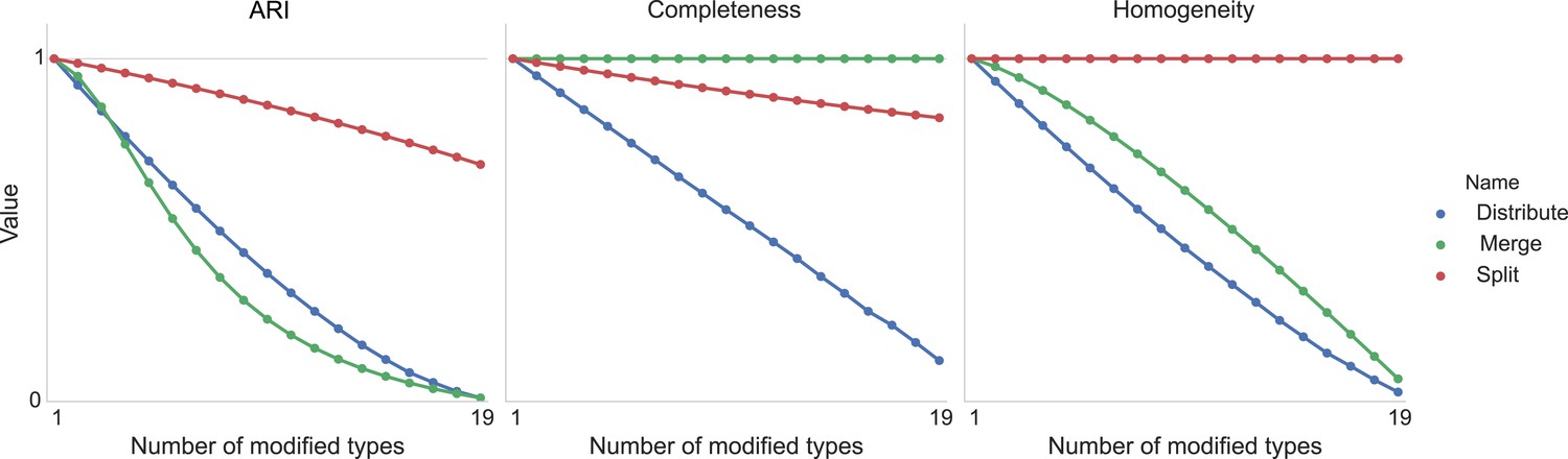
Type agreement evaluation metrics as a function of splitting types, merging types, and randomly distributing cells between types.
https://doi.org/10.7554/eLife.04250.013Download links
A two-part list of links to download the article, or parts of the article, in various formats.
Downloads (link to download the article as PDF)
Open citations (links to open the citations from this article in various online reference manager services)
Cite this article (links to download the citations from this article in formats compatible with various reference manager tools)
Automatic discovery of cell types and microcircuitry from neural connectomics
eLife 4:e04250.
https://doi.org/10.7554/eLife.04250


