Mapping microbial ecosystems and spoilage-gene flow in breweries highlights patterns of contamination and resistance
- University of California, Davis, United States
- University of Saskatchewan, Canada
Figures
Figure 1
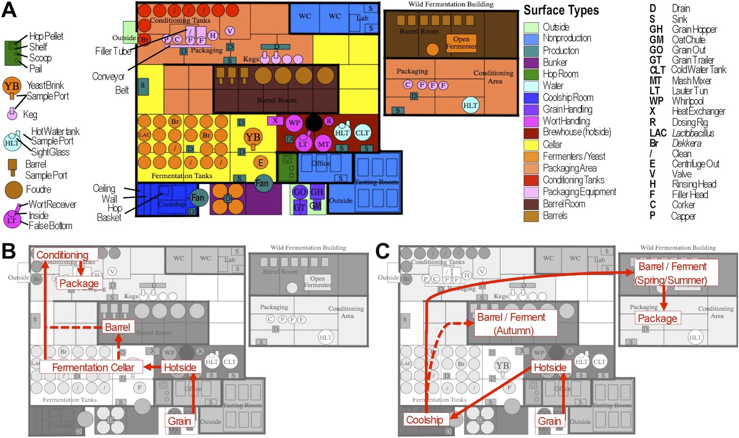
Brewery map and simplified brewing process diagrams.
(A) Floorplan of brewery details surface sampling key and indicates separate sections of the brewery. LAC/Br fermenters indicate they were inoculated intentionally with lactic acid bacteria or Dekkera spp., respectively, at the time of sampling. (B) Process diagram for conventional beer brewing, illustrating the relationship between brewing stages and sections of the brewery. Grain is milled and taken to the brewhouse (hotside) area where it is mashed (steeped in hot water) to form wort, which is lautered (extracted from the grain by filtering and spraying with hot water) and then boiled with hops. Boiled wort is cooled and pumped to the fermentation cellar where it is inoculated with Saccharomyces and fermented. Optionally, barrel-aged beers are transferred to barrels after fermentation. Finished beers are transferred to conditioning tanks in a separate section of the brewery where they are cooled, carbonated, and then packaged. (C) Process diagram for coolship beer brewing. Same as conventional, but following boiling wort is pumped to the coolship room where it is left to cool overnight, exposed to the atmosphere. The following morning, the wort is pumped to barrels in which it is fermented and aged for 1–3 years. In the Autumn samples, this occurred in the barrel room in the main brewery, but in Spring and Summer this moved to a newly built facility dedicated to sour beers. All coolship and sour beers were packaged on separate equipment in this second facility. The distinction between coolship beers and sour beers is the use of this coolship; other sour beers are produced using conventional brewing methods (panel B), but are fermented with organisms other than Saccharomyces yeasts.
Figure 2
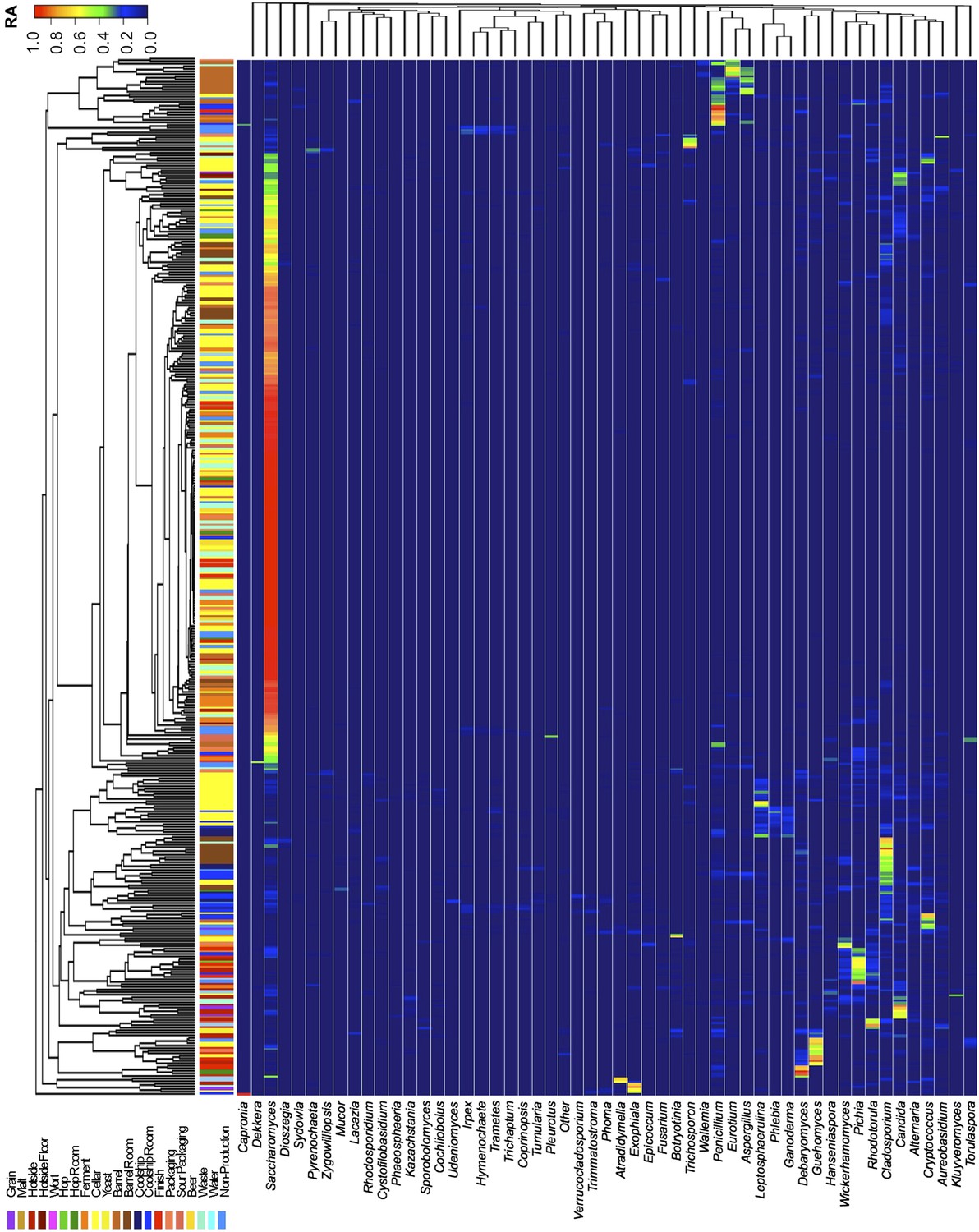
Taxon abundance heatmaps depict genus-level relative abundance of fungi across sampling sites detected by marker-gene sequencing.
The relative abundances (RA) of each genus (columns) within each sample (rows) are indicated by the color of the intersecting tile. Sample types are indicated by colored bars to the left of each row, classified according to the location within the brewery (Figure 1) or the type of substrate (grain, wort, hops, beer). Dendrograms represent Bray–Curtis dissimilarity between samples (vertical trees) and shared-niche similarity between taxa (horizontal trees), respectively indicating taxonomic composition similarities and taxon co-occurrence patterns. Only taxa ≥0.05 relative abundance in at least one sample are shown.
Figure 3
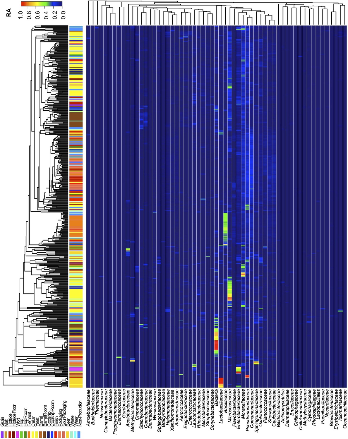
Taxon abundance heatmaps depict family-level relative abundance of bacteria across sampling sites detected by marker-gene sequencing.
The relative abundances of each genus (columns) within each sample (rows) are indicated by the color of the intersecting tile. Sample types are indicated by colored bars to the left of each row, classified according to the location within the brewery (Figure 1) or the type of substrate (grain, wort, hops, beer). Dendrograms represent Bray–Curtis dissimilarity between samples (vertical trees) and shared-niche similarity between taxa (horizontal trees), respectively indicating taxonomic composition similarities and taxon co-occurrence patterns. Only taxa ≥0.05 relative abundance in at least one sample are shown.
Figure 4
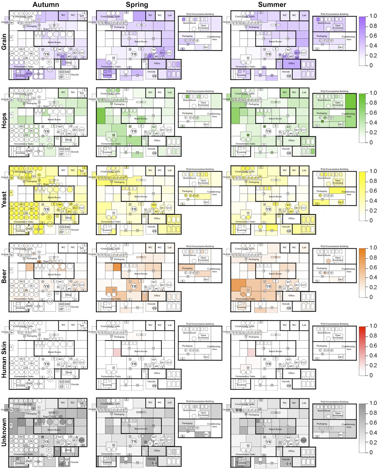
Mapping microbial contamination sources inside the brewery.
Floorplans of brewery indicate the predicted relative contamination of brewery surfaces by microbial sources (grains, hops, yeast, beer, human skin, unknown) at each season, estimated by SourceTracker (Knights et al., 2010). Coloration of each surface indicates the relative degree of microbial contamination from that source type (as indicated by keys to the right of each row; units are relative abundance). Contamination from outdoor air, soil, feces, freshwater, ocean water, and saliva was negligible (<0.001 relative abundance) and are not shown. See Figure 1 for a floorplan key and description of surfaces.
Figure 5
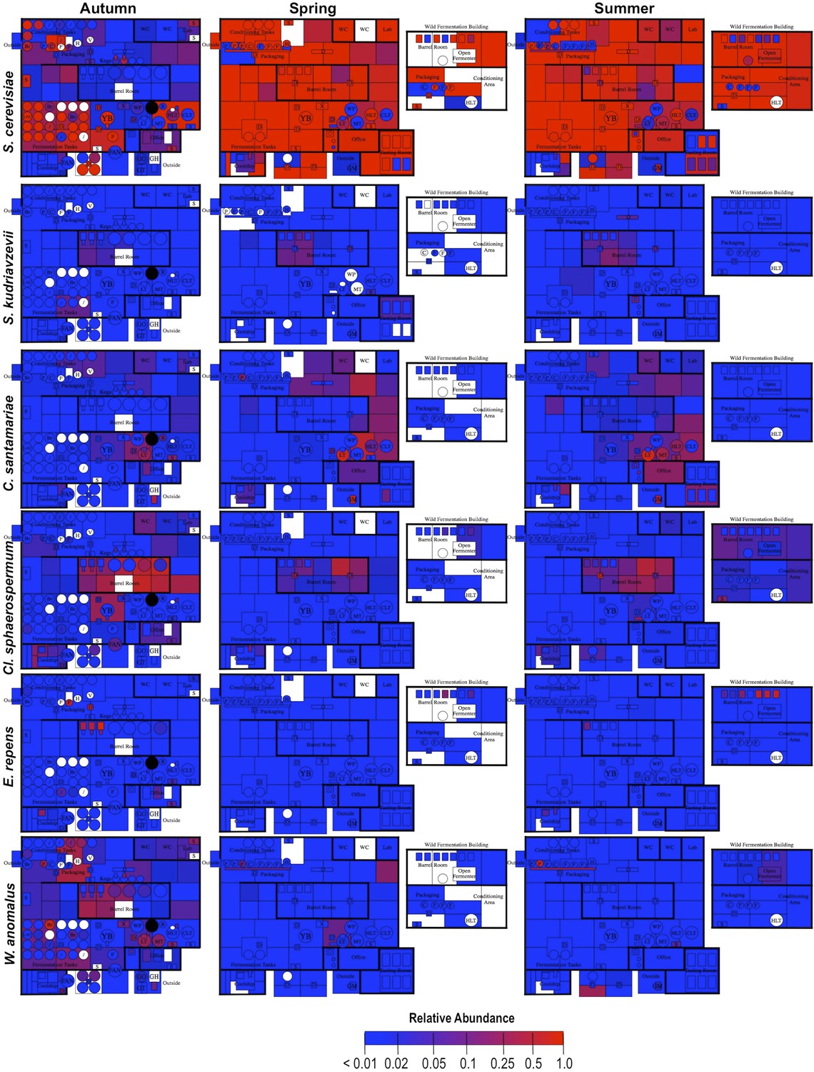
Spatial distribution heatmaps of fungi in brewery environments across seasons.
Plots indicate relative abundance of fungal taxa detected by ITS sequence reads across brewery surfaces at different times: Autumn (left), Spring (center), and Summer (right). See Figure 1 for a floorplan key and description of surfaces. Note that the floorplans change between seasons as some samples were only collected as specific timepoints and the wild brewing facility was built and opened during the Spring sampling time.
Figure 6
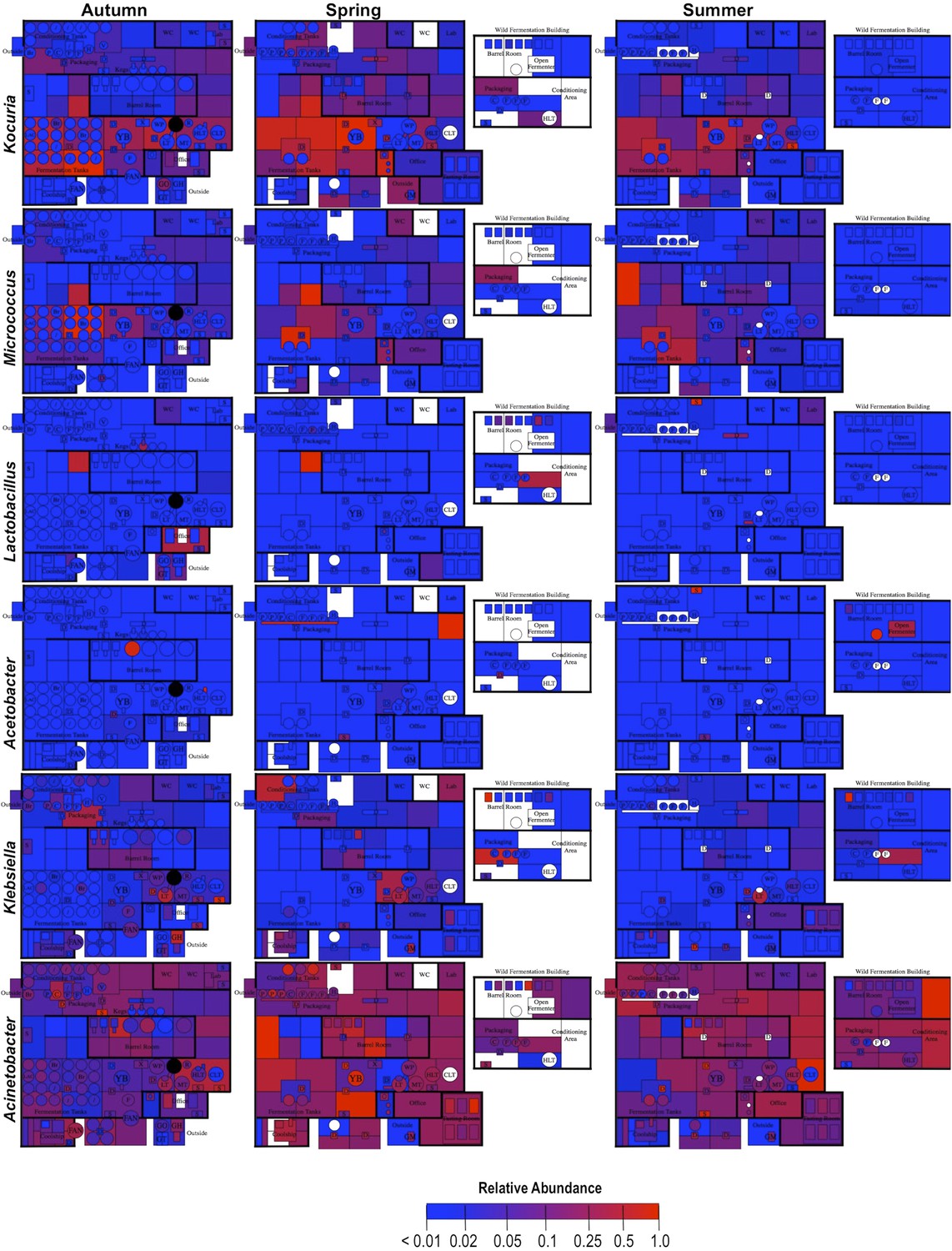
Spatial distribution heatmaps of bacteria in brewery environments across seasons.
Plots indicate relative abundance of bacterial taxa detected by 16S rRNA gene sequence reads across brewery surfaces at different times: Autumn (left), Spring (center), and Summer (right). Scales on right represent relative abundance scale (maximum 1.0) for each row of plots. See Figure 1 for a floorplan key and description of surfaces. Note that the floorplans change between seasons as some samples were only collected as specific timepoints and the wild brewing facility was built and opened during the Spring sampling time.
Figure 7
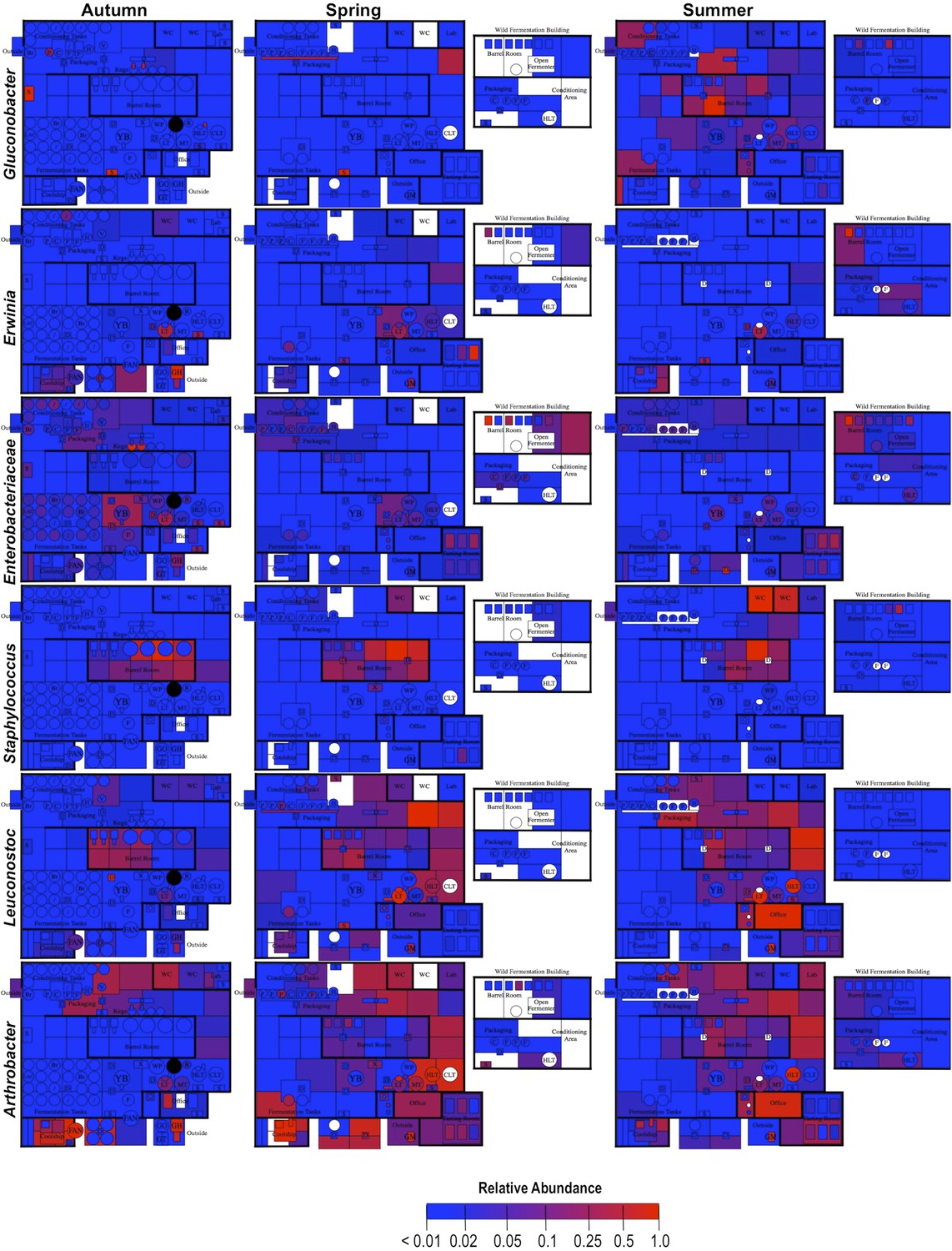
Spatial distribution heatmaps of bacteria in brewery environments across seasons (part 2).
Plots indicate relative abundance of bacterial taxa detected by 16S rRNA gene sequence reads across brewery surfaces at different times: Autumn (left), Spring (center), and Summer (right). Scales on right represent relative abundance scale (maximum 1.0) for each row of plots. See Figure 1 for a floorplan key and description of surfaces. Note that the floorplans change between seasons as some samples were only collected as specific timepoints and the wild brewing facility was built and opened during the Spring sampling time.
Figure 8
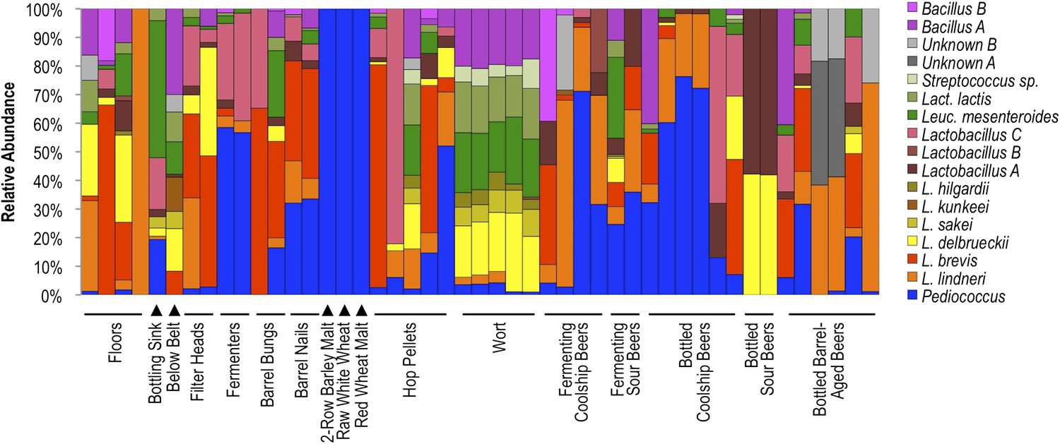
Lactic acid bacterial community composition on brewery surfaces, beers, and ingredients.
LAB-TRFLP profiles of samples exhibiting high Lactobacillales relative abundance by 16S rRNA gene sequencing.
Figure 9

Hop-resistance gene frequency on brewery surfaces and beers.
(A) ddPCR detection of hitA, horA, horB, and horC on surfaces (detected as copies/cm2) and in beers (copies/ml). Bar height indicates cumulative log gene abundance; colors indicate relative gene frequencies superimposed on these bars. Two barrel bung (stopper) samples are depicted on the left, one has no detection. (B) Pearson product-moment correlation matrix between hop-resistance genes, Lactobacillales relative abundance by 16S rRNA gene sequencing, and relative abundance of the dominant lactic acid bacteria detected by LAB-TRFLP. The color and shape of correlation ellipses (lower-left) indicate Pearson's product-moment correlation coefficient (r) between intersecting variables, as depicted in the key to the right. Correlations with larger positive r values are depicted as darker blue with increasingly narrow, upward-pointing ellipses. Correlations with larger negative r values are depicted as darker red with increasingly narrow, downward-pointing ellipses. Weaker correlations are depicted as wider, lighter colored ellipses. The corresponding p values for all correlation tests are provided in the reflected intersection (top-right).
Tables
Table 1
Hop-Resistance Gene Primers and Probes for ddPCR
| Target | Tm* | 5′ Label | Probe | Forward primer | Reverse primer | bp† |
|---|---|---|---|---|---|---|
| horB | 59 | FAM | TCGCGGCCAAGTGATACTTATCCTGA | AGTCGACACAAAATCCTGAATCA | AGCCTTGATCAATCGTCAGAC | 88 |
| hitA | 59 | HEX | ACAGAATAACGGCAACCAGTGTCGCAA | TCCTGTTGCTTCTGATGAAATTGG | CCGCTAAGAATACTTCGTAGGTGA | 105 |
| horA | 59.6 | FAM | CGCCGTTCCGCTCGTCTTGATCTGCC | TGGACTGGCGGATGACTATC | CTGTCTCGCTCTGGCAAC | 104 |
| horC | 59.6 | HEX | ACCACGCCAATGCCACTAGAAGCATGG | ACACGGTTAATGGCACAGC | GTTCGCGCCATAAAATAAGAGAGG | 87 |
-
*
Tm = melt temperature (°C).
-
†
Nucleotide length (bp).
Download links
A two-part list of links to download the article, or parts of the article, in various formats.
Downloads (link to download the article as PDF)
Open citations (links to open the citations from this article in various online reference manager services)
Cite this article (links to download the citations from this article in formats compatible with various reference manager tools)
Mapping microbial ecosystems and spoilage-gene flow in breweries highlights patterns of contamination and resistance
eLife 4:e04634.
https://doi.org/10.7554/eLife.04634


