Ambiguities in helical reconstruction
- University of Virginia, United States
Figures
Figure 1

The three-dimensional power spectrum of a helical filament and power spectra from projections of the filament.
The three-dimensional power spectrum of a helical filament is shown (A). The power spectrum from a cryo-EM image of a helical filament (where the image is a projection of a three-dimensional object onto a two-dimensional plane) is the central section of the three-dimensional power spectrum, and this would be given by the intersection of the red plane in (B) with the power spectrum. The yellow arrows in (B) show the intersection of this plane with a layer plane that arises from a 1-start helix. The intensities on this central section are shown in (D), which would be the power spectrum from untilted filaments, i.e., those whose filament axis is parallel to the plane of projection. The yellow arrow in (D) shows the layer line from the 1-start helix, with peak intensities on both sides of the meridian. Now consider what happens when the filament axis is tilted away from parallel to the plane of projection. The central section (C) would now intersect the 1-start layer plane at the positions given by the two yellow arrows, and in the two-dimensional power spectrum the two peaks would collapse to a single peak on the meridian (E, yellow arrow). If one did not know that the filament was tilted, such intensity would be mistaken for a meridional layer line with the Bessel order n = 0.
Figure 2
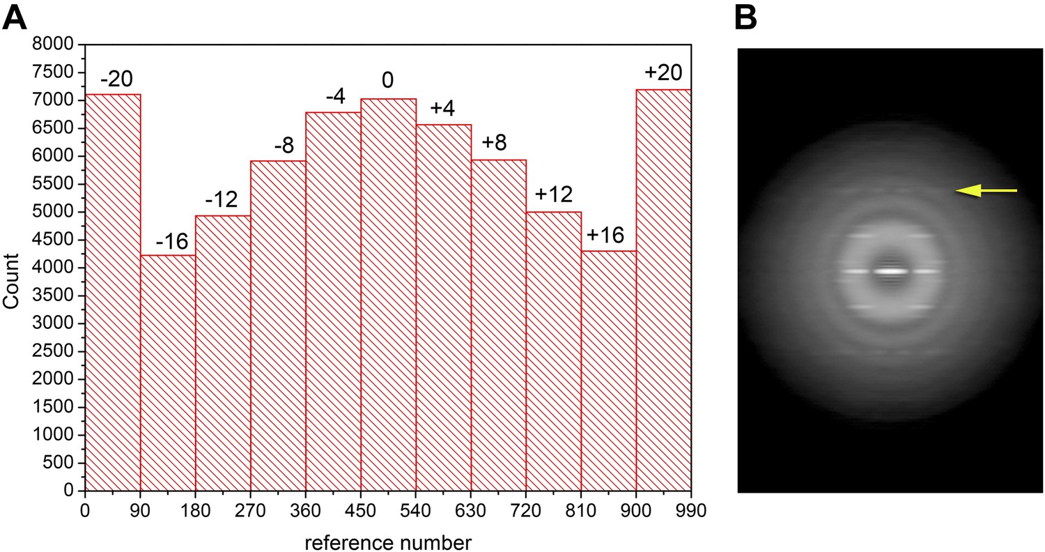
Out-of-plane tilt cannot be ignored in the images of Xu et al.
A histogram (A) of the out-of-plane tilt seen in the filaments of Xu et al. A reconstruction was generated from these filaments while allowing for out-of-plane tilt, and this reconstruction was used as a reference, generating 90 different azimuthal projections (4° increments) for tilt angles from −20° to +20° (also with 4° increments), generating 990 reference projections. The large peaks at both ends of the distribution arise from truncating the search range to smaller values than actually found in the filament population. Using filament segments in the three central bins (−4°, 0°, 4°) for generating a power spectrum (B) it can be seen that there is no meridional intensity on the layer line indicated by the arrow at ∼1/(18 Å), and the appearance of this layer line is now the same as in Wu et al. The log of the power spectrum is shown to better display the large dynamic range.
Figure 3
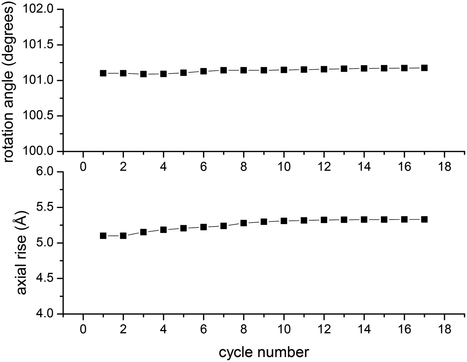
In the IHRSR method, the helical parameters (rotation and rise per subunit) are refined each cycle.
The starting parameters were the symmetry determined by Wu et al., and it can be seen that when using the images of Xu et al. these parameters are perfectly stable. The first seven cycles were run with images decimated from 2.3 Å/px to 4.6 Å/px, ignoring out-of-plane tilt. The subsequent cycles were run with the undecimated images and allowing for out-of-plane tilt.
Figure 4
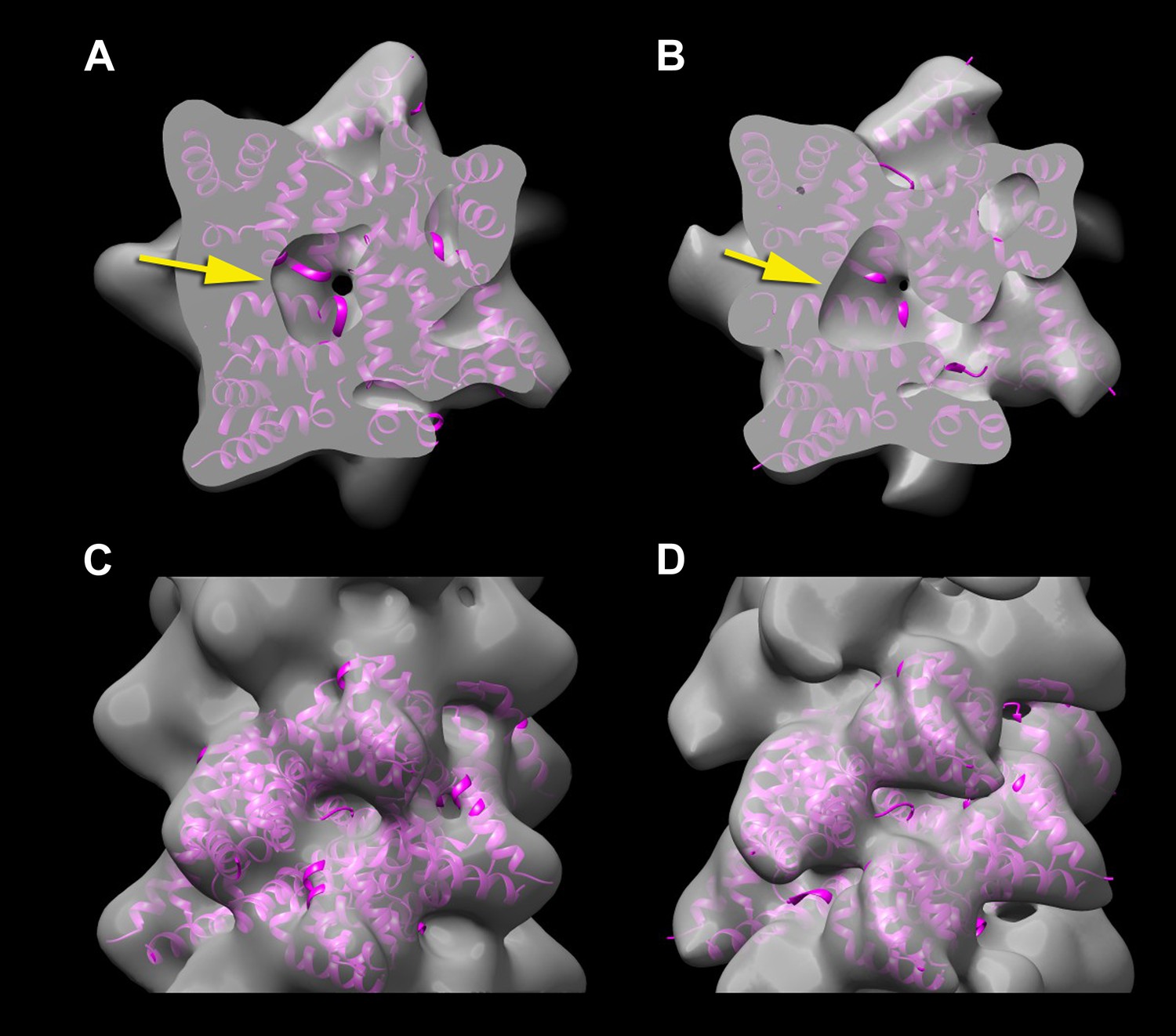
A reconstruction has been made from the filaments of Xu et al.
(A and C) by applying the helical symmetry described in Wu et al. For purposes of comparison, the reconstruction of Wu et al. (EMDB-5922) has been filtered to 12 Å resolution (B and D). It can be seen that with similar thresholds, both reconstructions show a hole in the center (A and B, arrows), arising from the helical procession of the subunits about the filament axis. The atomic model (3J6J.PDB) from Wu et al. (2014) is shown fit into both reconstructions.
Figure 5
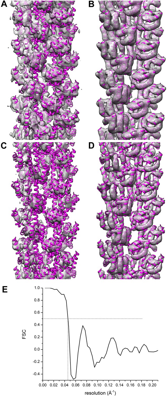
Comparisons between a model and the actual map are informative.
The reconstruction (A and C) of Xu et al. (EMDB-5890) is compared with their model 3j6c.PDB (B and D). In all four panels (A–D) the same model (3j6c.PDB) is shown as magenta ribbons, but the transparent surfaces in B and D have been generated by filtering the model density to 9.6 Å, the stated resolution of the reconstruction shown in (A and C). The surfaces in (C and D) are shown at a higher threshold than in (A and B). It can be seen that with these thresholds, there is virtually no correlation between the map (A and C) and the model (B and D). A Fourier Shell Correlation between their model and reconstruction (E) shows that at FSC = 0.5 the resolution is ∼22 Å, which is consistent with the visual comparison of the map and model (A–D).
Download links
A two-part list of links to download the article, or parts of the article, in various formats.
Downloads (link to download the article as PDF)
Open citations (links to open the citations from this article in various online reference manager services)
Cite this article (links to download the citations from this article in formats compatible with various reference manager tools)
Ambiguities in helical reconstruction
eLife 3:e04969.
https://doi.org/10.7554/eLife.04969


