A genuine layer 4 in motor cortex with prototypical synaptic circuit connectivity
- Northwestern University, United States
- University College London, United Kingdom
Figures
Figure 1
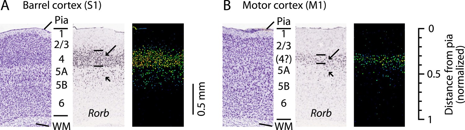
L4 in M1 as a zone of Rorb expression.
Images are from the Allen Mouse Brain Atlas (http://mouse.brain-map.org/) (Lein et al., 2007) showing coronal sections for Rorb in situ hybridization (probe Rorb-RP_071018_01_H03) and corresponding Nissl stains. (A) S1 labeling. In a Nissl-stained section (left), L4 is readily identifiable due to cell density differences across layers. In situ hybridization labeling of Rorb (center, with corresponding expression intensity image shown on the right) is the strongest in L4 (long arrow, with borders indicated by lines), with weaker labeling present in L5A/B (short arrow). (B) M1 labeling. Nissl stain (left) showing a region of the lateral agranular cortex corresponding to the forelimb representation area of M1 (same section as in panel A). L4 is not readily identifiable based on cell density differences alone. Nevertheless, in situ hybridization against Rorb (center and right) shows the strongest labeling in a laminar zone corresponding to L4 in S1 (long arrow, with borders indicated by lines), with weaker labeling present in L5A/B (short arrow). Scale on the far right shows the normalized cortical distance from pia to white matter (WM). The approximate location of the cortical layers is indicated, based on prior quantitative analysis of the bright-field optical appearance of M1 layers (Weiler et al., 2008).
Figure 2
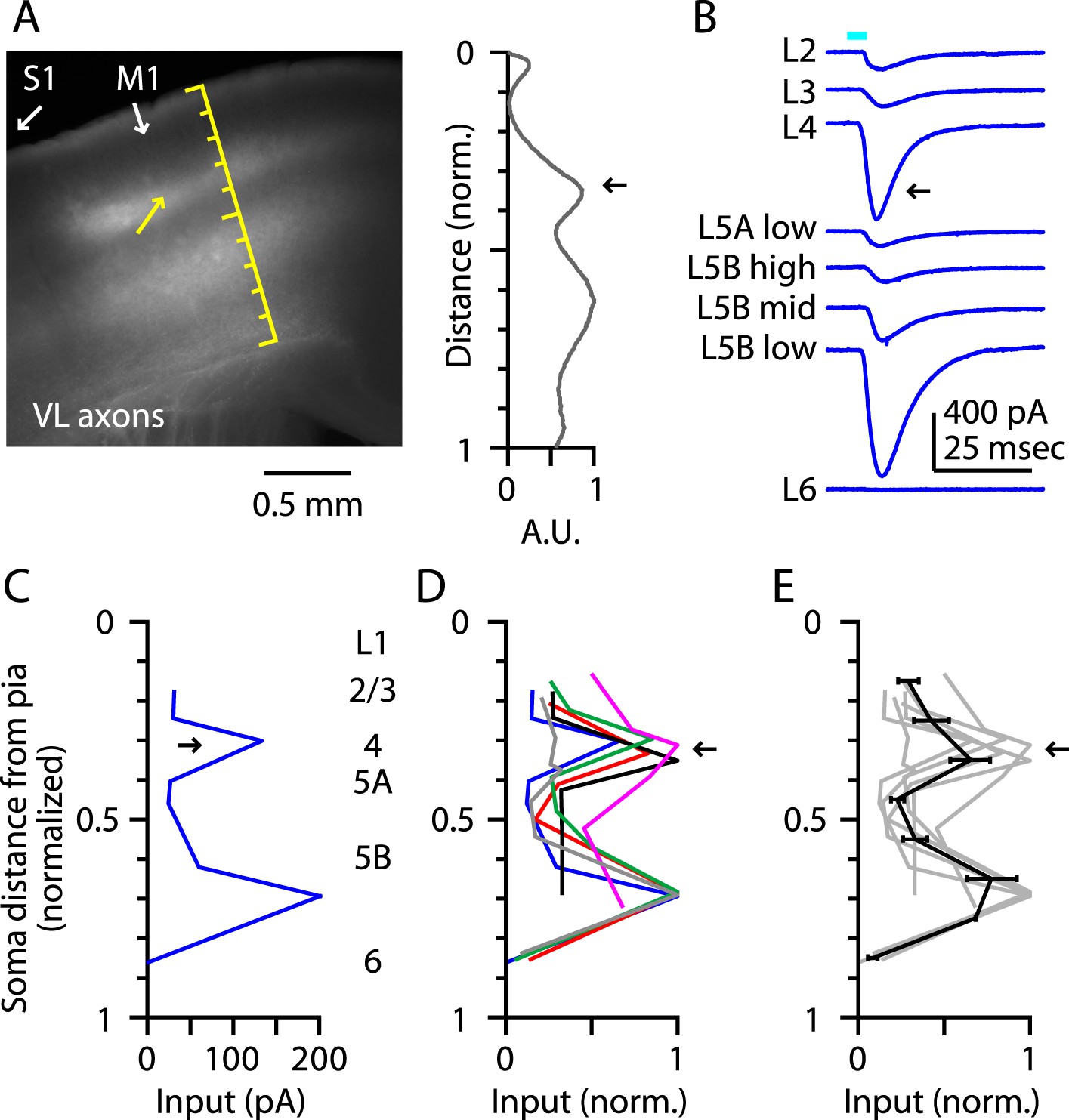
Thalamocortical (TC) input to M1-L4 neurons from VL.
(A) Epifluorescence image of coronal slice containing M1, showing laminar pattern of labeled thalamocortical axons following injection of AAV carrying ChR2 and GFP in the ventrolateral (VL) region of the thalamus. S1 cortex is located laterally (to the left, as indicated). Scale shows normalized cortical distance. Yellow arrow indicates laminar zone of labeling where strong photostimulation-evoked electrophysiological responses were also detected. Plot to the right shows laminar profile of fluorescence intensity, in arbitrary units (A.U.), across layers (normalized distance from pia). (B) Responses recorded (sequentially) in vitro in multiple M1 neurons in different layers (as indicated) to photostimulation of ChR2-labeled axons originating from motor thalamus (VL) neurons (Hooks et al., 2013). (C) Laminar profile of VL input to M1 neurons. The profile exhibits two peaks, one in the upper ∼1/3 of the cortex (corresponding to L4) and the other in the lower part (corresponding to L5B). (D) Laminar profiles obtained from multiple slices (n = 6). Most profiles show a clear peak at a normalized depth of ∼1/3 (black arrow). (E) Average laminar profile (black; bars: s.e.m.), calculated by binning the data for each profile (bin width: 1/10 of the normalized cortical depth), averaging within each bin, and then averaging across all profiles. The individual profiles are also shown (gray).
Figure 3
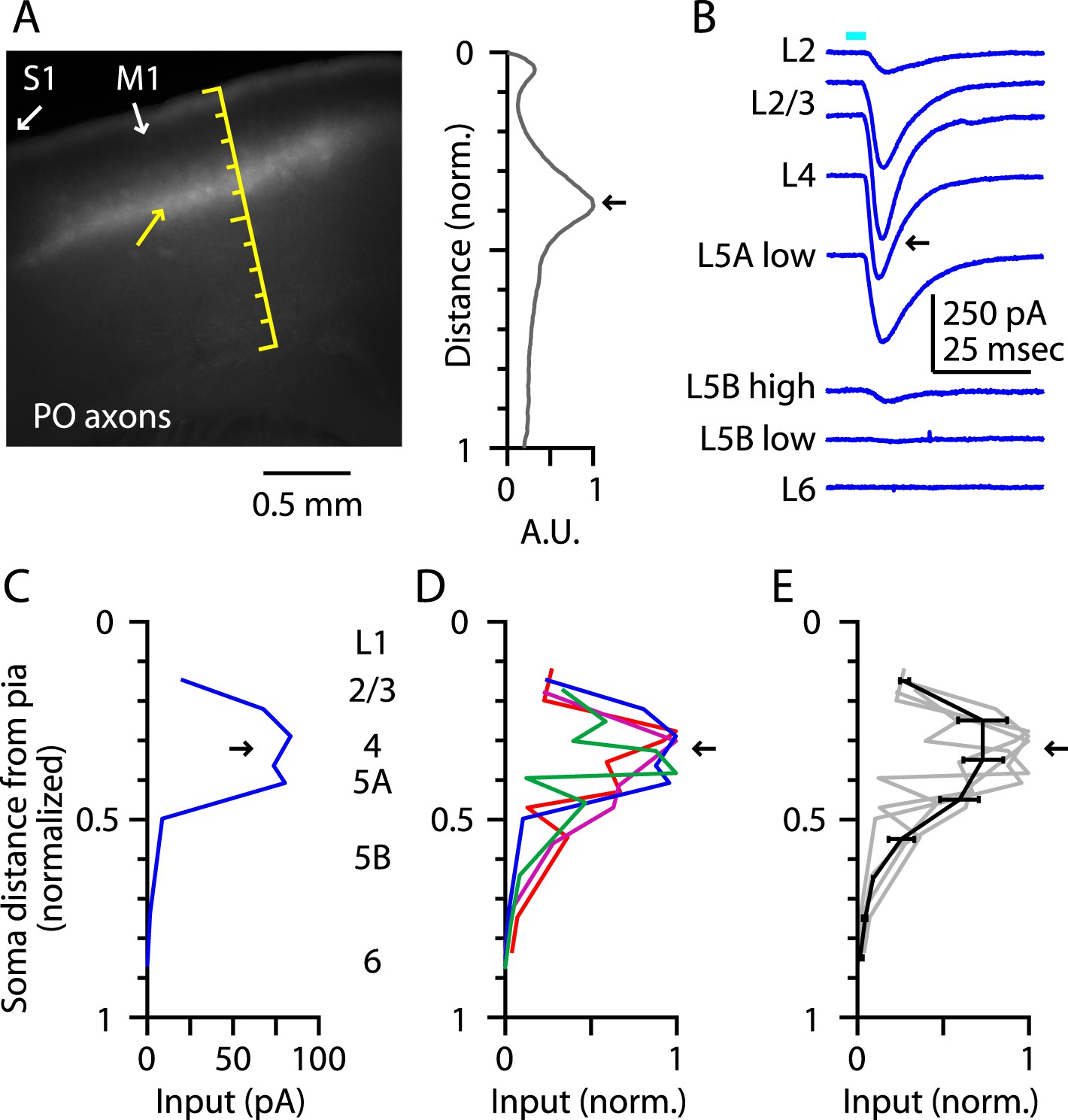
Thalamocortical (TC) input to M1-L4 neurons from PO.
(A) Epifluorescence image of coronal slice containing M1, showing laminar pattern of labeled thalamocortical axons following injection of AAV carrying ChR2 and GFP in the PO region of the thalamus. S1 cortex is located laterally (to the left, as indicated). Scale shows normalized cortical distance. Yellow arrow indicates laminar zone of labeling where strong photostimulation-evoked electrophysiological responses were also detected. Plot to the right shows laminar profile of fluorescence intensity, in arbitrary units (A.U.), across layers (normalized distance from pia). (B) Responses recorded (sequentially) in vitro in multiple M1 neurons in different layers (as indicated) to photostimulation of ChR2-labeled axons originating from sensory thalamus (posterior nucleus; PO) neurons (Hooks et al., 2013). (C) Response amplitudes of the same neurons plotted as a function of laminar location, providing a laminar profile of VL input to M1 neurons. The profile exhibits one peak, situated in the upper ∼1/3 of the cortex, somewhat wider (vertically) compared with the peak of VL input, spanning the laminar zone corresponding to L4. (D) The laminar profiles obtained from multiple slices (n = 4). Profiles show a broad peak at a normalized depth of ∼0.2–0.5 (black arrow). (E) Average laminar profile (black; bars: s.e.m.), calculated by binning the data for each profile (bin width: 1/10 of the normalized cortical depth), averaging within each bin, and then averaging across all profiles. The individual profiles are also shown (gray).
Figure 4

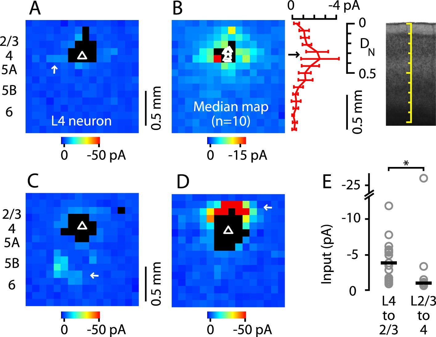
Excitatory output from M1-L4 neurons to L2/3.
(A) Top: bright-field image of a parasagittal slice containing motor (M1) and somatosensory (S1) cortex. In S1, L4 barrels are easily discernable, but are absent from M1, where L5A (lighter-appearing laminar zone) appears wider than in S1. Graduated scale indicates cortical depth in normalized units, from the pia (0) to the white matter (1). Yellow boxes indicate placement of photostimulation grid for mapping inputs to L2/3 neurons in both cortical areas. Bottom: Schematic indicating the major areas and layers of interest in the image. (B) Example of a synaptic input map recorded in a L2/3 neuron in M1. Grid spacing was set to 75 µm, the top of the grid was flush with the pial surface, and the grid was horizontally centered over the soma (triangle). Cortical layers indicated to the left, with the location of the L3/5A border (as observed under bright-field) marked by a horizontal line. Inputs arise from both this L4-like laminar zone and the lateral sites in L2/3. Photosimulation sites where the postsynaptic neuron's dendrites were directly stimulated were excluded from analysis and are shown as black pixels. (C) Example of a synaptic input map recorded in a L2/3 neuron in S1. Same mapping parameters as in B. The input pattern is similar to that of the M1 example shown in B, but with weaker L2/3 and stronger ascending input from the subjacent region corresponding to the L4 barrel layer. (D): Mean input map for M1 neurons (n = 14). The laminar profile (plotted to the right of the map; red, M1; gray, S1) shows a peak at the level of the L3/5A border (black arrow), ∼0.5 mm deep, corresponding to ∼1/3 of the normalized cortical depth (DN) in both M1 and S1. The bottom plot shows the L4 region of the same plot, with the input profiles normalized (IN) to their peak values in L4 (arrow); the scaled M1 profile closely resembles the S1 profile. (E): Mean input map for S1 neurons (n = 13).
Figure 5
Paucity of local input to M1-L4 neurons from L2/3 and other layers.
(A) Example of a typical synaptic input map recorded from a M1-L4 neuron, showing mostly intralaminar excitatory input (arrow), and little L2/3 input. The triangle marks the location of the soma, and the black pixels represent photostimulation sites resulting in direct dendritic responses. (B) Median input map for M1-L4 neurons (n = 10). Excitatory input arose mostly from intralaminar sources, with notably little from L2/3 sites. The laminar profile (plotted to the right of the map; red, median ± median absolute deviation; gray, individual cells) shows a peak at the level of the L3/5A border, ∼0.5 mm deep, corresponding to ∼1/3 of the normalized cortical depth (DN). (C) A M1-L4 neuron showing both intralaminar sources of excitation and ascending excitation from L5B/6 sites (arrow). (D) An exceptional M1-L4 neuron. (E) Comparison of the individual (gray circles) and median (black lines) amplitudes of L4 input to M1-L2/3 neurons vs L2/3 input to M1-L4 neurons (*p < 0.05, rank-sum test).
Figure 6
M1-L4 neurons receive and send relatively little long-range corticocortical input.
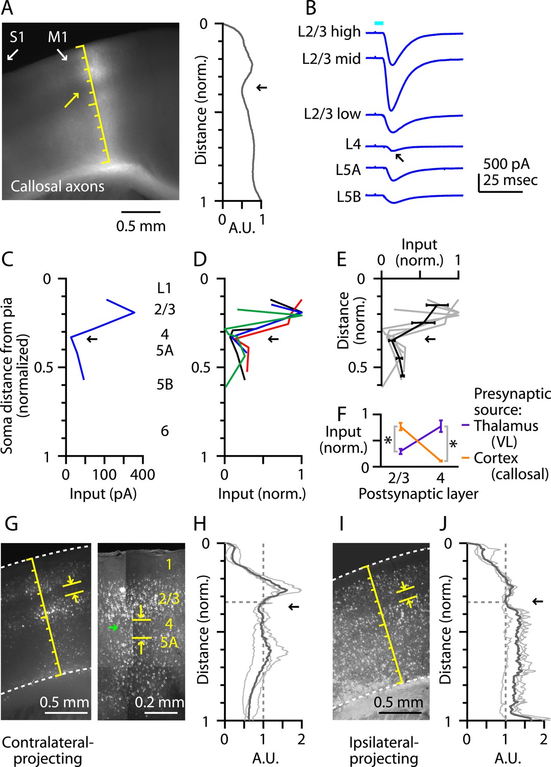
(A) Epifluorescence image of coronal slice containing M1, showing laminar pattern of labeled interhemispheric corticocortical axons following injection of AAV carrying ChR2 and GFP in the contralateral M1. Scale shows normalized cortical distance. Arrow indicates laminar zone of labeling where weakest photostimulation-evoked electrophysiological responses were also detected. Plot to the right shows laminar profile of fluorescence intensity, in arbitrary units (A.U.), across layers (normalized distance from pia). (B) Responses recorded (sequentially) in vitro in multiple M1 neurons in different layers (as indicated) to photostimulation of ChR2-labeled axons of contralateral M1 neurons infected with AAV-ChR2. (C) Response amplitudes of the same neurons plotted as a function of laminar location, providing a laminar profile of contralateral M1 input to M1 neurons. The profile exhibits a dip in the upper ∼1/3 of the cortex (corresponding to L4) (arrow). (D) The laminar profiles were obtained from multiple slices (n = 4). Profiles show a dip ∼1/3 deep in the cortex (in normalized coordinates). (E) Average laminar profile (black; bars: s.e.m.), calculated by binning the data for each profile (bin width: 1/10 of the normalized cortical depth), averaging within each bin, and then averaging across all profiles. The individual profiles are also shown (gray). (F) Comparison of input from callosal axons (from contralateral M1; n = 4 slices) vs thalamic axons (from VL; n = 6 slices), recorded in postsynaptic L2/3 and L4 neurons in M1 (*p < 0.01, rank-sum test). For each slice, values within each laminar zone (in units of normalized cortical depth: L2/3, 0.1 to 0.25; L4, 0.29 to 0.37) were averaged to obtain a single value per profile; these were averaged and plotted with error bars representing the s.e.m. (G) Representative epifluorescence image (left) showing gap (marked by yellow arrows) at the level of L4 (∼1/3 deep in the cortex, in normalized distance units) in the retrograde labeling of M1 neurons following injection of retrograde tracers in contralateral M1. Two-photon microscopic image (right) showing the same labeling pattern at a higher resolution (different animal). Some neurons within the ‘gap’ are labeled with the retrograde tracer (green arrow). (H) Laminar profiles of fluorescence intensity of M1 neurons projecting to contralateral M1. Each trace represents the average profile for one animal, obtained by averaging several M1-containing slices. For display, the profiles were normalized to the value in L4 (specifically, the value at a normalized cortical depth of 1/3). The bold line is the average of three animals. There is a reduction in labeling intensity in the L4 region (arrow). (I) Representative epifluorescence image showing gap at the level of L4 in the retrograde labeling of M1 neurons following injection of retrograde tracers into ipsilateral M2, S1, and S2. (J) Laminar profiles of retrograde labeling pattern for ipsilateral injections. Average traces were calculated as in Panel G. The average (bold line) of three animals shows a zone of reduced labeling observed ∼1/3 deep in the cortex, corresponding to L4 (arrow).
Figure 7

Electrophysiological properties of M1-L4 cells.
(A) Resting membrane potential (Vr), plotted as a function of the cortical depth of the soma (normalized distance from pia). A total of 56 neurons were sampled across layers 2/3 through 5A. For analysis, neurons were binned into three main laminar groups corresponding to L2/3, L4, and L5A. The blue lines indicate the laminar range of each group, and also represent their mean ± s.e.m. values. Significant differences between groups are marked (*, rank-sum test). See ‘Materials and methods’ for additional details. (B) Input resistance (Rinput) vs soma depth. (C) Action potential (AP) width vs soma depth. (D) AP amplitude vs soma depth. (E) (Vthresh − Vr) vs soma depth. (F) Current (I) threshold vs soma depth. (G) Rinput vs Ithresh. (H) Slope of the frequency–current (F–I) relationship. (I) Spike-frequency adaptation (SFA) ratio. (J) Example traces, representing the various types of repetitive firing patterns observed among L4 neurons.
Figure 8
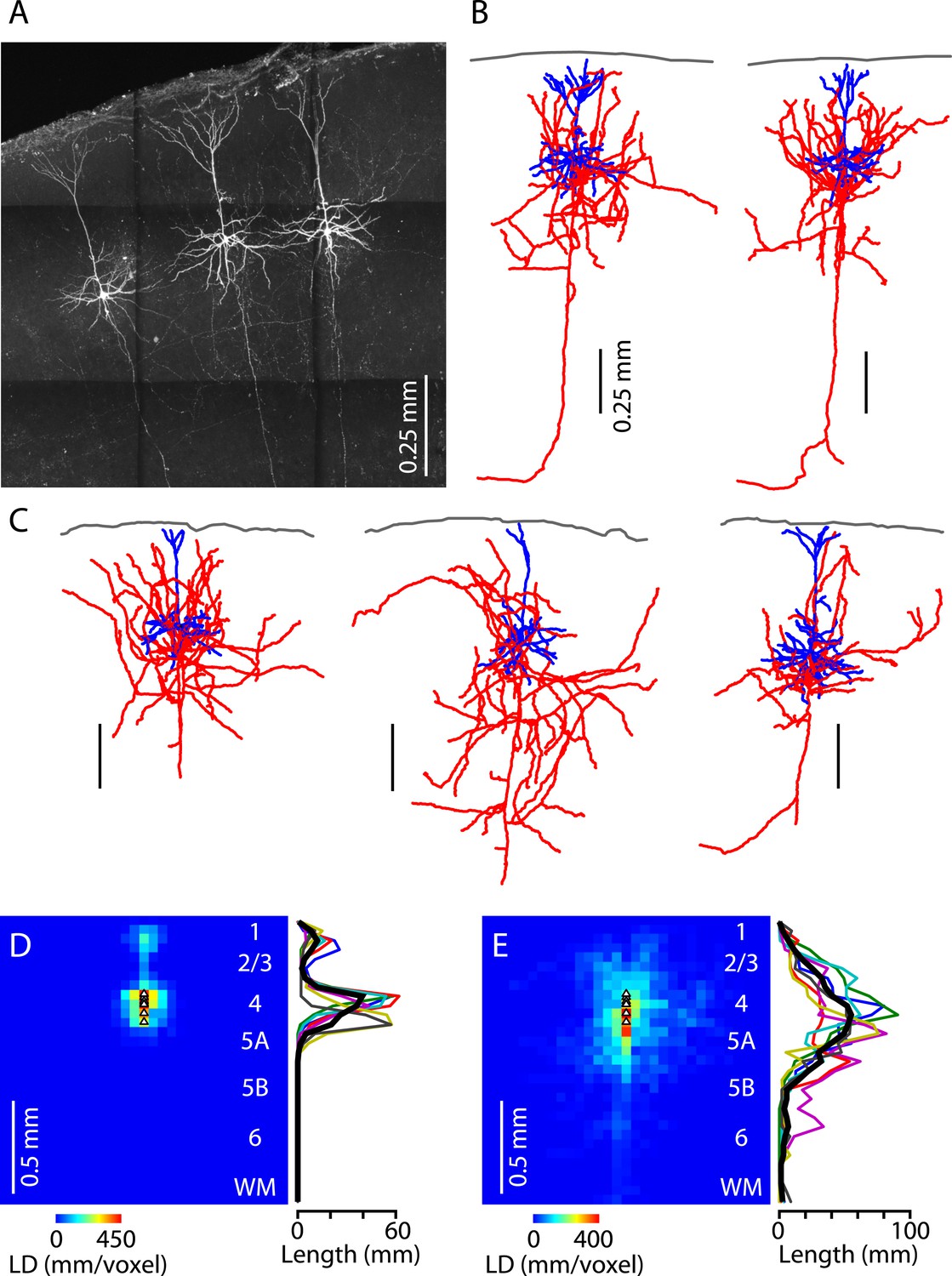
Morphological properties of M1-L4 neurons.
(A) Example fluorescence image of M1-L4 neurons. The neurons were filled with biocytin during whole-cell recordings, fixed and fluorescently labeled, and imaged with a two-photon microscope. The image is a maximum-intensity projection of multiple aligned image stacks. (B) Three-dimensional reconstructions of the two L4 neurons in the center and right of the image are shown in panel A. Dendrites are blue, axons are red, and the pia is drawn across the top. (C) Three more examples. (D) Quantitative analysis of dendritic morphology. The three-dimensional digital reconstructions (n = 6 neurons) of L4 neurons' dendrites were converted to two-dimensional length–density maps and averaged. Plot to the right shows the same data as a vertical profile (black: group mean ± s.e.m.; colored lines, individual neurons). (E) Same analysis, for the axons of the same neurons.
Tables
Table 1
Electrophysiological properties of L2/3, L4, and L5A neurons in M1
| Parameter | L2/3 neurons (n = 15) | L4 neurons (n = 18) | L5A neurons (n = 8) | L2/3 vs L4 | L4 vs L5A | L2/3 vs L5A |
|---|---|---|---|---|---|---|
| Vr (mV) | −78 ± 1 | −72 ± 1 | −69 ± 2 | *0.00079 | 0.089 | *0.00095 |
| Rinput (Mohm) | 65 ± 4 | 71 ± 7 | 148 ± 17 | 0.99 | *0.00095 | *0.00034 |
| Cm (pF) | 146 ± 12 | 109 ± 11 | 90 ± 7 | 0.038 | 0.42 | *0.0061 |
| Sag (%) | 2.8 ± 0.3 | 4.3 ± 0.6 | 6.0 ± 1.0 | 0.057 | 0.13 | *0.0088 |
| f-I slope (Hz/nA) | 63 ± 4 | 80 ± 8 | 103 ± 16 | 0.12 | 0.19 | *0.0045 |
| Ithresh (pA) | 267 ± 19 | 295 ± 26 | 163 ± 23 | 0.45 | *0.0030 | *0.0038 |
| SFA ratio | 0.89 ± 0.02 | 0.89 ± 0.02 | 0.74 ± 0.05 | 0.91 | *0.0054 | *0.0080 |
| Vthresh (mV) | −33 ± 1 | −35 ± 1 | −32 ± 1 | 0.19 | 0.21 | 0.85 |
| AP amplitude (mV) | 72 ± 2 | 79 ± 2 | 66 ± 2 | *0.015 | *0.00078 | 0.028 |
| AP width (msec) | 1.21 ± 0.08 | 0.98 ± 0.01 | 1.03 ± 0.02 | *0.0060 | 0.23 | 0.19 |
| Vthresh − Vr (mV) | 46 ± 2 | 38 ± 2 | 37 ± 2 | * 0.00028 | 0.32 | * 0.0041 |
-
Values under each cell group are mean ± s.e.m. Numbers in the last three columns are p-values for comparisons between the indicated groups (rank-sum test; asterisks indicate significant differences). Vr, resting membrane potential; Rinput, input resistance; Cm, cell capacitance; Ithresh, current threshold for evoking action potential(s); SFA ratio, spike-frequency accommodation ratio; Vthresh, voltage threshold for action potential; AP amplitude, action potential peak minus threshold; AP width, action potential duration. See ‘Materials and methods’ for additional details.
Additional files
-
Source code 1
Custom Matlab routines for length density analysis of neuronal morphology.
- https://doi.org/10.7554/eLife.05422.012
Download links
A two-part list of links to download the article, or parts of the article, in various formats.
Downloads (link to download the article as PDF)
Open citations (links to open the citations from this article in various online reference manager services)
Cite this article (links to download the citations from this article in formats compatible with various reference manager tools)
A genuine layer 4 in motor cortex with prototypical synaptic circuit connectivity
eLife 3:e05422.
https://doi.org/10.7554/eLife.05422


