Distinct effects of prefrontal and parietal cortex inactivations on an accumulation of evidence task in the rat
- NYU Shanghai, China
- Princeton University, United States
- University of Washington, United States
- Howard Hughes Medical Institute, Princeton University, United States
Figures
Figure 1
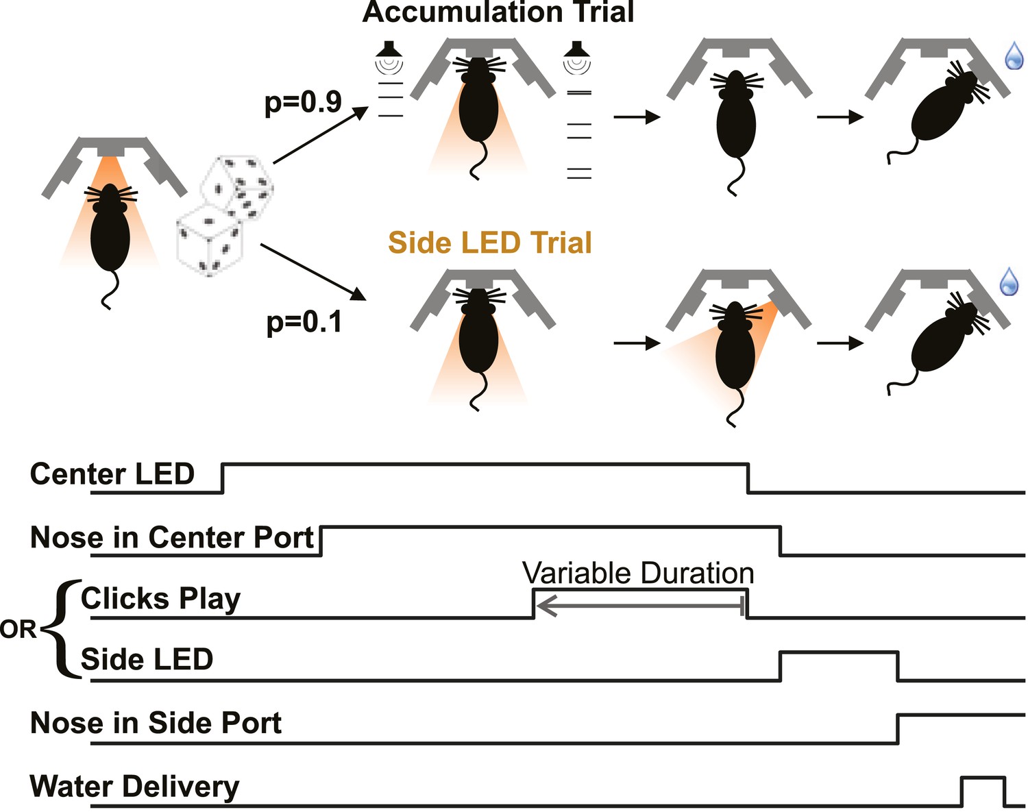
Poisson clicks accumulation task trials and interleaved side LED trials.
Each accumulation task trial begins with the onset of the center LED, which signals to the rat to enter the center port. The subject holds his nose in the center port for 2 s, until the center LED offset, which is the go cue. The majority of trials (90%) are accumulation trials. On accumulation trials, clicks play from the right and left speakers (right + left click rate = 40 clicks/s), terminating with the go cue. After the go cue reward is available at the side port associated with the greater number of clicks. The stimulus duration on each trial is set by the experimenter to be in the range 0.1–1 s. On Side LED trials, no sound is played during the fixation period and one of the side ports is illuminated once the rat withdraws from the center port to indicate that reward is available there. Accumulation and side LED trials are randomly interleaved, as are left and right trials.
Figure 2 with 2 supplements
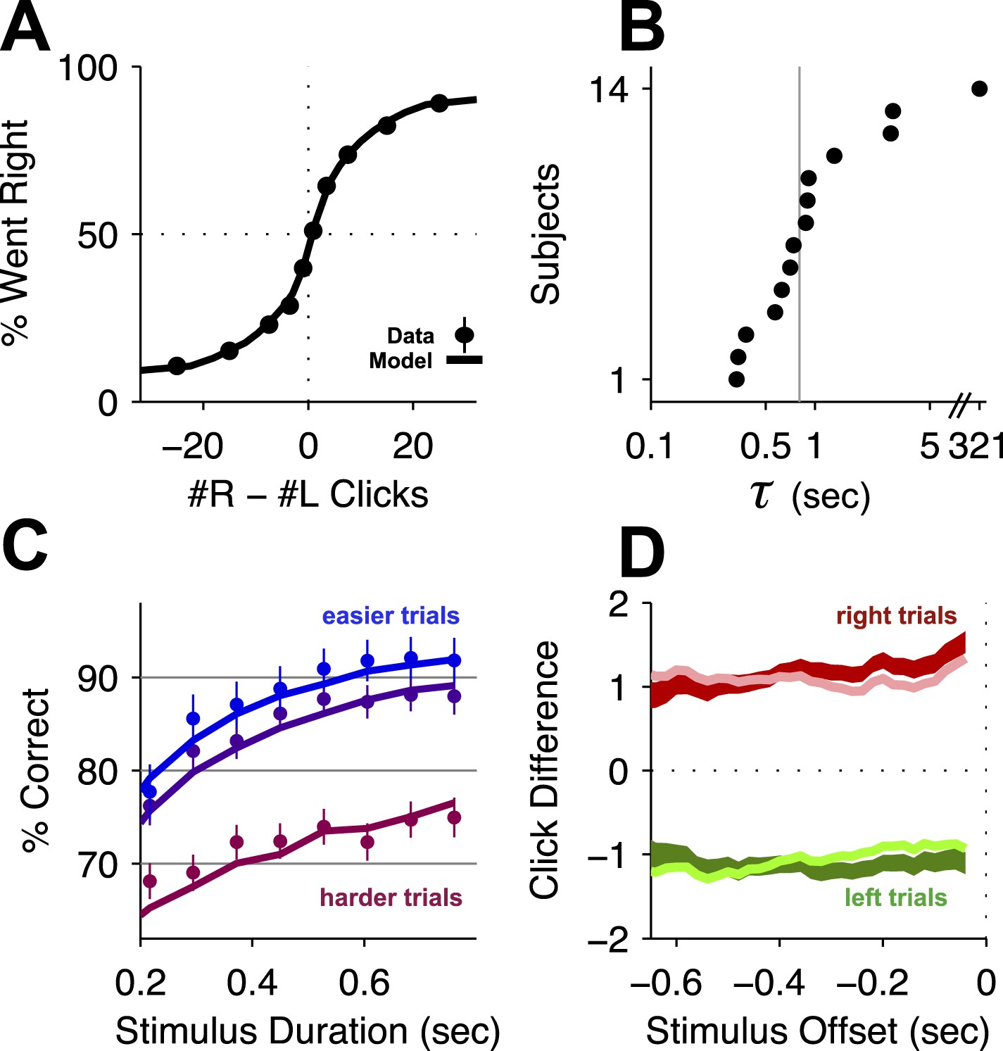
Behavioral evidence of accumulation.
(A) Behavior as a function of total right minus total left clicks. For very easy trials (large click differences) performance is ≈90% correct. The circles (with very small error bars) are the mean ±95% binomial confidence intervals across accumulator trials from all rats 1 day before an infusion session (n = 47,580 trials across 14 rats). The thick line is the psychometric curve generated by the accumulator model fit to these trials. (B) The time-constant of accumulation as fit by the model for each rat in the experiment. The median (810 ms) is marked by a thin gray line. (C) Chronometric plot generated using the same data as in panel (A). The rats' performance increases with longer duration stimuli, consistent with an accumulation strategy. The circles and error bars are the mean ±95% binomial confidence intervals across trials on the easiest (blue), middle (purple) and hardest (magenta) thirds of trials defined by the absolute value of the ratios of left vs right click rates. The thick lines are the model generated chronometric curves. (D) Reverse correlation analyses showing that clicks throughout the stimulus were used in the rats' decision process, supporting the long accumulation time constants in (B). The thick dark red and green lines are the means ± std. err. across trials for where the rats went right and left. Thin light red and green lines are the model generated reverse correlation.
Figure 2—figure supplement 1
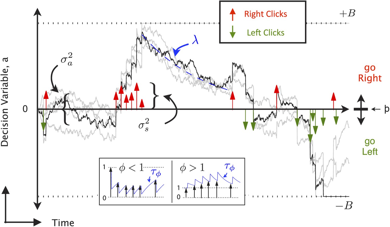
9-parameter Accumulator Model (reproduced from Brunton et al., 2013).
At each timepoint, the accumulator memory a (black trace) represents an estimate of the ‘Right’ vs ‘Left’ evidence accrued so far. At stimulus end, the model decides ‘Right’ if a > Þ, the decision boundary, and ‘Left’ otherwise, where Þ is a free parameter. Light grey traces indicate alternate runs with different instantiase.
a The decision variable. Right ↑ (left ↓) pulses change the value of a by positive (negative) impulses of magnitude C.
parameterizes noise in the initial value of a.
a diffusion constant, parameterizing noise in a.
parameterizes noise when adding the evidence from a Right or Left pulse: variance is added to the amplitude C of the evidence contributed by each click.
λ parameterizes consistent drift in the memory a. In the ‘leaky’ or forgetful case (λ < 0, illustrated), drift is towards a = 0, and later pulses impact the decision more than earlier pulses. In the ‘unstable’ or impulsive case (λ > 0), drift is away from a = 0, and earlier pulses impact the decision more than later pulses. The memory's time constant τ = 1/λ.
B the height of the ‘sticky’ decision bounds and parameterizes the amount of evidence necessary to commit to a decision.
φ, τϕ parameterize sensory adaptation by defining the dynamics of C. Immediately after a click, the magnitude C is multiplied by φ. C then recovers towards an unadapted value of 1 with time constant τϕ. Facilitation is thus represented by ϕ > 1, while depression is represented by ϕ < 1 (inset).
Þ the decision boundary. These properties are implemented by the following equations: if |a| ≥ B then da/dt = 0; else
(1)
where
δt,tR,L are delta functions at the times of the pulses.
η are i.i.d. gaussian variables drawn from .
dW is a white noise Wiener process.
The initial condition a(t = 0) is drawn from the gaussian .
Adaptation dynamics are given by:
(2)
In addition, a lapse rate parameterizes the fraction of trials on which a random response is made.
Ideal performance (a = #right clicks − #left clicks) would be achieved by Þ = 0.
© 2013 AAAS. All Rights Reserved. Figure 2—figure supplement 1 and legend text reproduced from Brunton BW, Botvinick MM, Brody CD. 2013. Rats and humans can optimally accumulate evidence for decision-making. Science 340, 95–98. doi:10.1126/science.1233912. Reprinted with permission.
Figure 2—figure supplement 2
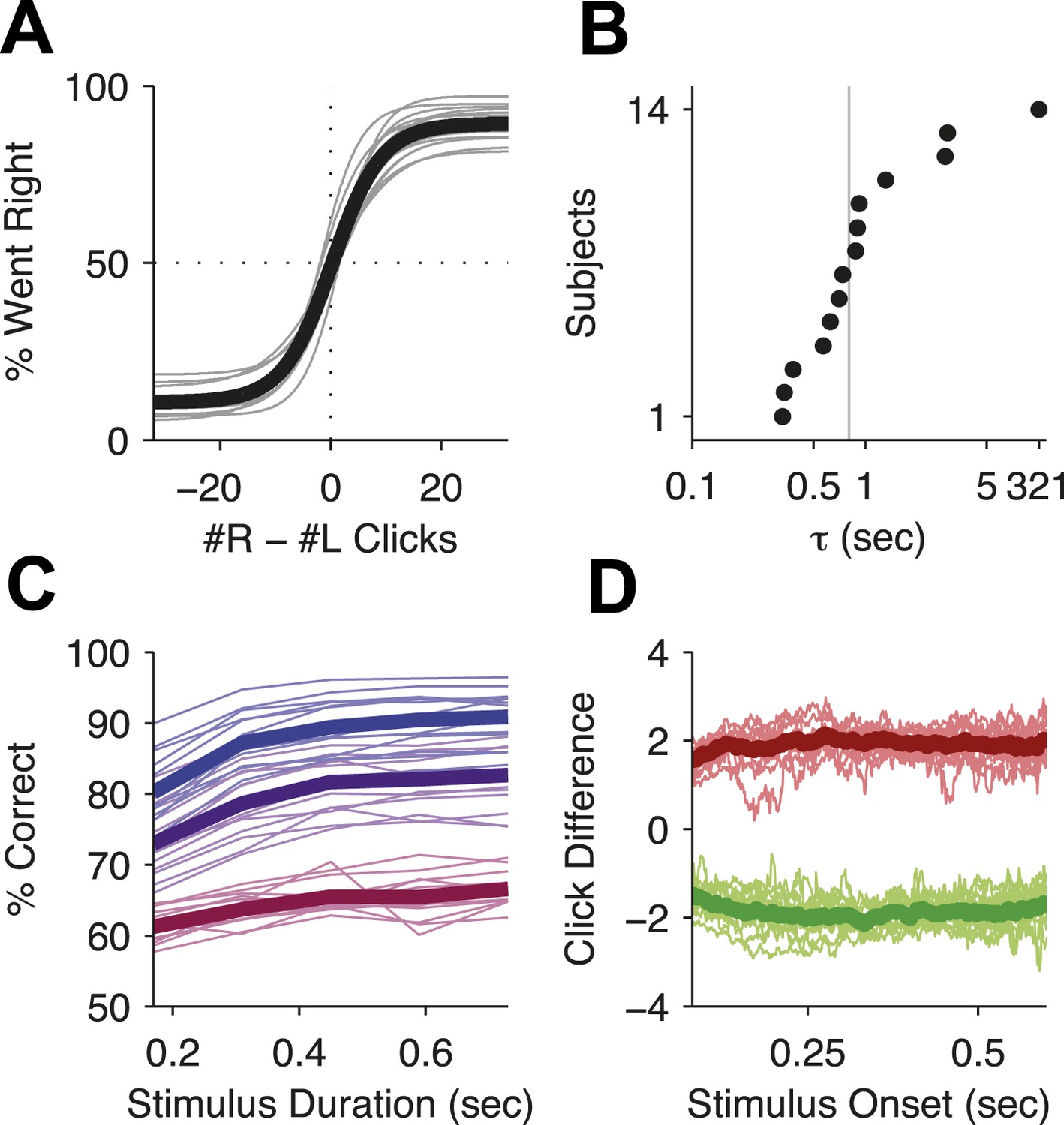
Behavioral evidence of accumulation in individual rats.
(A) Behavior as a function of total right minus total left clicks. For very easy trials (large click differences) performance is ≈90% correct. The thick line is the average performance of the 14 rats in the study, the thin gray lines are the performance of individual rats. (B) The time-constant of accumulation as fit by the model for each rat in the experiment. The median (810 ms) is marked by a thin gray line. (C) Chronometric plot showing that rats performance increases with longer duration stimuli, consistent with an accumulation strategy. The thin lines are the performance of individual rats (n = 14) on the easiest (blue), middle (purple) and hardest (magenta) thirds of trials defined by the absolute value of the ratios of left vs right click rates. The thick lines show the means across rats. (D) Reverse correlation analyses showing that clicks throughout the stimulus were used in the rats' decision process supporting the long accumulation time constants in (B). Thin light red and green lines are the reverse click rate correlation of individual rats (n = 14). The thick dark red and green lines are the means across rats.
Figure 3 with 3 supplements
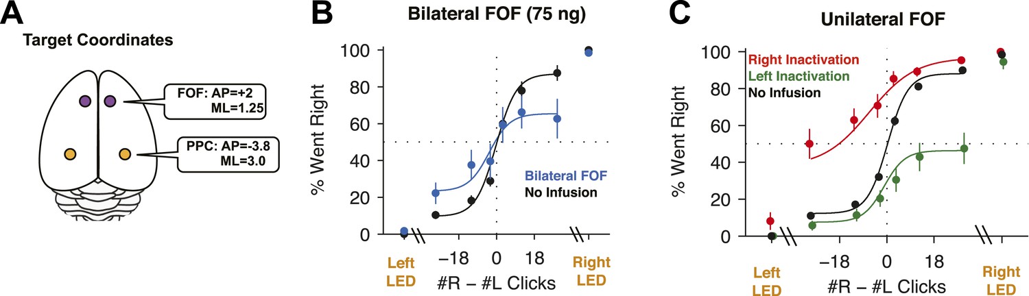
FOF Infusions.
(A) Top-down view of rat cortex with the locations of the FOF and the PPC, into which cannulae were implanted. (B) Bilateral infusion of muscimol into the FOF results in a substantial impairment on accumulation trials but has no effect on side LED trials. In black are data from control sessions 1 day before an infusion (n = 8 sessions, 4 rats). In blue are data from bilateral FOF infusions (n = 8 sessions, 4 rats, 75 ng per side). The circles with error bars indicate the mean ± s.e. across sessions. Accumulation trials are binned by #R − #L clicks, spaced so there are equal number of trials in each bin. The lines are a 4-parameter sigmoid fit to the data. (C) Unilateral infusion of muscimol into the FOF results in a profound ipsilateral bias on accumulation trials but has no effect on side LED trials. In black are data from control sessions 1 day before an infusion (n = 34 sessions, 12 rats). In red are data from right FOF infusions (n = 17 sessions, 12 rats, 150 or 300 ng). In green are data from left FOF infusions (n = 17 sessions, 12 rats, 150 or 300 ng).
Figure 3—figure supplement 1
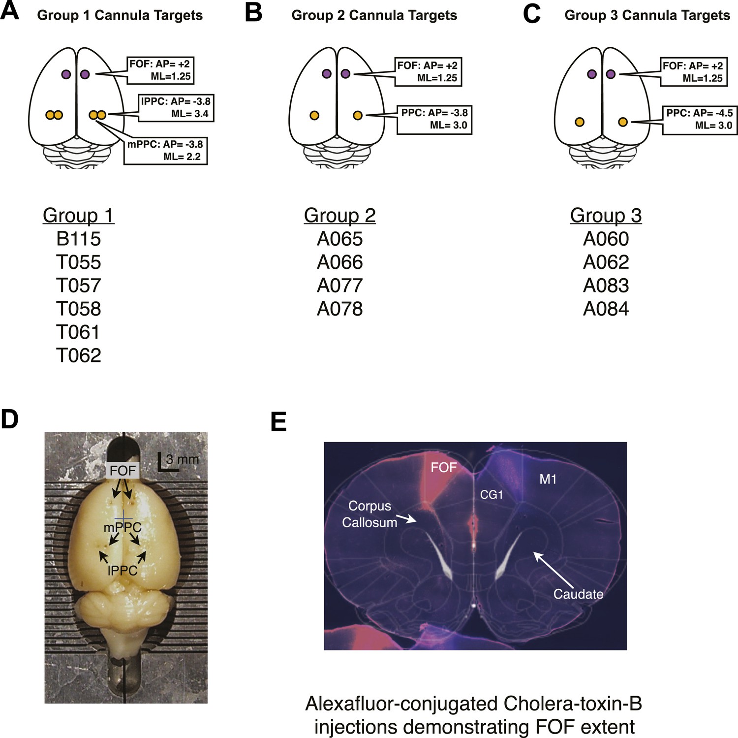
Cannula coordinates and histology.
(A–C) The targets of cannula implants for group 1,2, and 3 with the list of the rats in each group. (D) A birds-eye view of rat T061's brain after fixation and removal from the skull. The AP and ML locations of the cannula are clearly visible by eye. Each line of the brain blocker marks 1 mm. The blue cross marks the approximate location of Bregma. (E) Coronal section of a rat brain that had been infused through the implanted FOF cannula with two colors (‘red’ on the left and ‘blue’ on the right) of Alexa Fluor-conjugated cholera toxin-B subunit, a fluorescent tracer. The rat was perfused 1 week after infusion of tracer. The tracer has labelled cells along the AP axis of the FOF. Shown here is a section from 2.5 mm anterior to Bregma (Paxinos and Watson, 2004). Note, that in the nomenclature of Paxinos and Watson (2004) the area that we describe as the FOF is considered to be part of M2. In the bottom left corner, the top of another coronal section overlaps with the shown section.
Figure 3—figure supplement 2
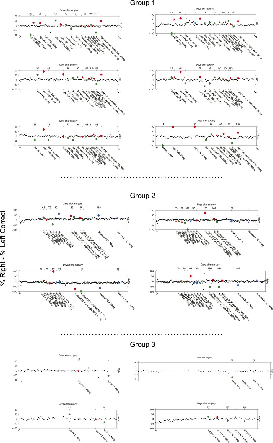
Timeline of bias for each rat.
Each point of the figure is the bias for a single session (%Right − %Left Correct). The number at the beginning of the x-axis indicates the days passed since surgical implantation with cannula. Control non-infusion days are shown as black dots. Right infusions are shown in red, Left infusions are shown in green. Bilateral infusions are shown in blue. For the simultaneous bilateral FOF and unilateral PPC infusions, the color indicates the side of the PPC infusion as in Figure 4C. Stars indicated PPC infusions, Diamonds indicate FOF infusions. Hollow markers indicate an infusion session where the subject did not perform enough trials to analyze. The bottom x-labels describe the details (side, region and dose) of each infusion. The top x-labels indicate the number of days passed from cannula surgery. If infusions generate an ipsilateral bias then red markers should be above zero and green markers below zero.
Figure 3—figure supplement 3

FOF infusions cause profound impairment in the clicks task.
The psychometric data and GLMM model fits for bilateral FOF infusions in each rat (n = 4). Open circles are binned data from accumulation trials and the small points are the predictions of the GLMM fits at sampled data points. (A) In black are the isoflurane control fits and in blue are the bilateral infusion fits. In every rat the slope of the bilateral infusions is shallower than in the isoflurane controls. In three of four rats there was also a shift, likely due to the challenge of performing perfectly balanced bilateral infusions. In three of four rats (All but A066) the difference between performance between bilateral FOF and isoflurane is significantly different. (B) The psychometric data and GLMM model fits for unilateral FOF infusions in each rat (n = 12). Open circles are binned data from accumulation trials and the small points are the predictions of the GLMM fits at sampled data points. In red are the right infusion data and fits and in green are the left infusion data and fits. In every rat the right infusions result in more rightward responses on accumulation trials than the left infusions.
Figure 4
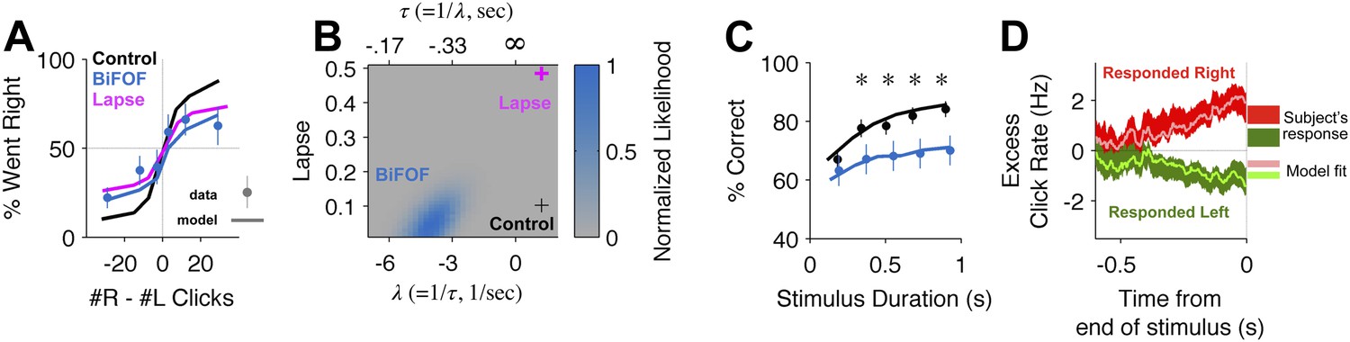
Bilateral FOF inactivation is best fit as a reduction in the time-constant of accumulation.
(A) When analyzed in terms of the psychometric function, changes to either lapse rate alone or accumulation time constant alone can match the bilateral FOF inactivation data. The black line shows the psychometric curve from control data, collected 1 day before bilateral FOF sessions (n = 1526 trials). Blue dots with error bars show the experimental data from bilateral FOF inactivation sessions (n = 1809 trials). The magenta line is the psychometric curve obtained by fitting only the lapse rate parameter to the inactivation data, while keeping all other parameters at their control values (corresponds to magenta cross in panel B). The blue line shows the psychometric curve from the accumulator model fit to the inactivation data (corresponds to peak of blue likelihood surface in panel B), which has a change w.r.t. control in accumulation time constant τ (=1/λ), but no change in lapse rate. (B) Fitting the detailed click-by-click, trial-by-trial accumulator model (Brunton et al., 2013) to the inactivation data clearly distinguishes between lapse and λ. The panel shows the normalized likelihood surface, indicating quality of the model fit to the inactivation data as a function of the lapse and the λ (=1/τ) parameters. The black cross shows parameter values for the control data. The best fit to the inactivation data is at the peak of the blue likelihood surface (λ = −4.15, lapse = 0.048), significantly different from control for λ, but not different from control for lapse. This best-fit lambda corresponds to λ = −0.241 s, a substantially leaky integrator. (C) Performance as a function of stimulus duration for bilateral FOF sessions (blue, mean ± std. err.) and the control sessions 1 day before (black, mean ± std. err.). The lines are the chronometric curves generated by the accumulator model (for inactivation data, parameter values at peak of blue likelihood surface in panel B). (D) Reverse correlation showing the relative contribution of clicks from different times to the rats' decisions for data from bilateral FOF inactivation sessions. Compare to Figure 2D. The thick dark shading shows the mean ± std. err. across trials based on the rats' choices. The thin bright lines are the reverse correlation traces generated by the accumulator model (parameter values at peak of blue likelihood surface in panel B).
-
Figure 4—source data 1
MATLAB file containing resampled bilateral FOF model fits.
This MATLAB file contains three variables. BF: a 300 × 9 matrix. Each row is the set of parameters which maximized the likelihood of the accumulator model fit to a resampling of the bilateral FOF data. Each column is a parameter. LL: a 300 × 1 vector with the negative log likelihood of the corresponding row of BF. parameter_names: a 9 × 1 cell with the names of the columns of BF.
- https://doi.org/10.7554/eLife.05457.012
Figure 5
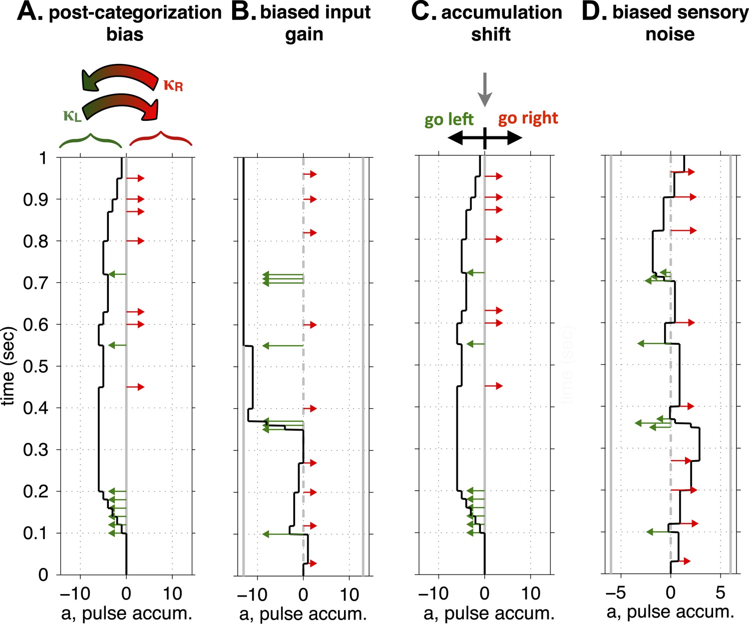
Conceptual illustration of four model parameters, used to quantify different sources of a lateralized bias.
(A) Post-categorization bias: after categorizing the accumulator value into ‘Go Left’ or ‘Go Right’ decisions, a fraction, κL, of Left decisions are reversed into Right decisions, and a fraction, κR, are reversed from Right to Left. (B) Biased input gain, which can be thought of as a form of sensory neglect: Left and Right clicks have different impact magnitudes on the value of the accumulator. In this illustration left clicks have a much stronger impact, and decisions will consequently be biased to the left. (C) Accumulation shift: before categorizing the accumulator into ‘Go Left’ vs ‘Go Right’ decisions (by comparing the accumulator's value to 0), a constant is added to the value of the accumulator. (D) Biased sensory noise, which by differentially affecting signal-to-noise rations from the two sides, can be thought of as a form of sensory neglect distinct from biased input gain: Left and Right clicks have different magnitudes of noise in their impact. In this illustration, left clicks are more variable than right clicks, which biases decisions to the right.
Figure 6 with 2 supplements

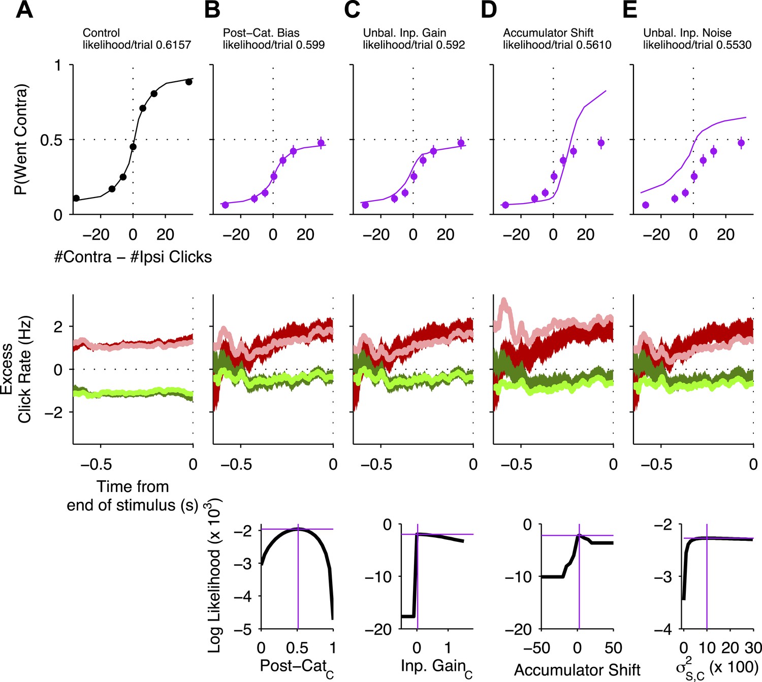
Unilateral FOF inactivation is best fit as a post-categorization bias.
(A) A comparison of the likelihoods (i.e., best model fits) for the four different bias mechanisms illustrated in Figure 5. The post-categorization bias model is better than the next best model (biased input gain) by 50 log-units. (B) The 2-dimensional normalized likelihood surface for the two best single-parameter models: post-categorization bias and input gain bias. For visualization, we plot the contra-ipsi bias for the two parameters. That is, the difference between the contralateral and ipsilateral values for each parameter. The y-axis is κC − κI. The x-axis is CC − CI. By definition, in the control model (black marker) these biases are 0. The peak of the magenta likelihood surface for the inactivation data is significantly different from control for post-categorization bias (from 0 to 0.4588) but not significantly different from control for input gain bias. (C) Psychometric curves for control and inactivation data. The black line is the model fit to the control data (see Figure 2A for the data points). The magenta circles with error bars are experimental data from unilateral FOF inactivation sessions, and indicate fraction of Contra choice trials (mean ± binomial 95% conf. int.) across trial groups, with different groups having different #Contra − #Ipsi clicks. The magenta line is the psychometric curve generated by the post-categorization bias model. (D) Performance as a function of stimulus duration for data from control sessions 1 day before (black), and for data from unilateral FOF sessions (magenta, mean ± std. err.). The lines are the chronometric curves generated by the corresponding model (E) Reverse correlation analyses showing the relative contributions of clicks throughout the stimulus in the rats' decision process. The thick dark red and green lines are the means ± std. err. across trials for contralateral and ipsilateral trials. Thin light red and green lines are the reverse correlation traces generated by the post-categorization bias model. (F) Psychometric curves for single-sided trials in control (black), right FOF infusion (red) and left FOF infusion (green) sessions, demonstrate that even for very easy trials FOF infusions produce a vertical scaling, consistent with post-categorization bias.
Figure 6—figure supplement 1
Psychometric and reverse correlation comparisons of data and model for unilateral FOF inactivations.
Top row: For all curves, the circles with error bars indicate fraction of Contra choice trials (mean ± se) across trial groups, with different groups having different #Contra − #Ipsi clicks. The lines are model fits that differ from the control data in a single parameter (see main text). Magenta data points in (B–E) are data from unilateral FOF infusions. Middle row: Reverse correlation analyses showing the relative contributions of clicks throughout the stimulus in the rats' decision process. The thick dark red and green lines are the means ± std. err. across trials for contralateral and ipsilateral trials. Thin light red and green lines are the reverse correlations predicted by the same accumulator models that were used to plot psychometric fits in corresponding column of the top row. Bottom Row: Likelihood as a function of model parameter value. This demonstrates that there was a single global maximum for each 1-parameter model. The magenta cross in each plot indicates the best-fit value of the corresponding parameter (on the x-axis) and the log likelihood of that model (on the y-axis) and corresponds to the model used to generate the psychometric curve and reverse correlations in the top and middle rows. (A) Data (black circles) from control sessions 1 day before an infusion session and a 9-parameter accumulator model fit (line). (B) Post-categorization bias model. (C) Unbalanced Input model. (D) Accumulator Shift model. (E) Unbalanced input noise model.
Figure 6—figure supplement 2

Distribution of sample from 8-parameter model of unilateral FOF inactivation.
Using the Metropolis–Hastings algorithm we collected 40,000 samples from an 8-parameter model of the unilateral FOF inactivation. The parameters are the rows and columns of this matrix of plots. The histograms along the diagonal show the marginal distributions of individual parameters which were used to non-parametrically assess whether individual parameters were significantly different from control values. Each other plot is a scatter plot that gives an estimate of the marginal distribution for each pair of parameters. From left to right: λ and are the accumulation parameters from the original 9-parameter model. , I is the variance associated with ipsilateral clicks. The accumulator shift parameter is labeled bias here, as in the original model. Post-CatI (i.e., κI) is the proportion of ipsilateral choices that are flipped to contralateral choices. , C is the variance associated with contralateral clicks. GainC is the amplitude of contralateral clicks (i.e., CL). Ipsilateral clicks are assigned a gain of 1. Post-CatC (i.e., κC) is the proportion of contralateral choices that are flipped to ipsilateral choices. Note the plot showing the 2D marginal distribution of Post-CatC vs GainC shows the same shape as the likelihood surface in Figure 6B, validating the sampling method.
Figure 7 with 1 supplement
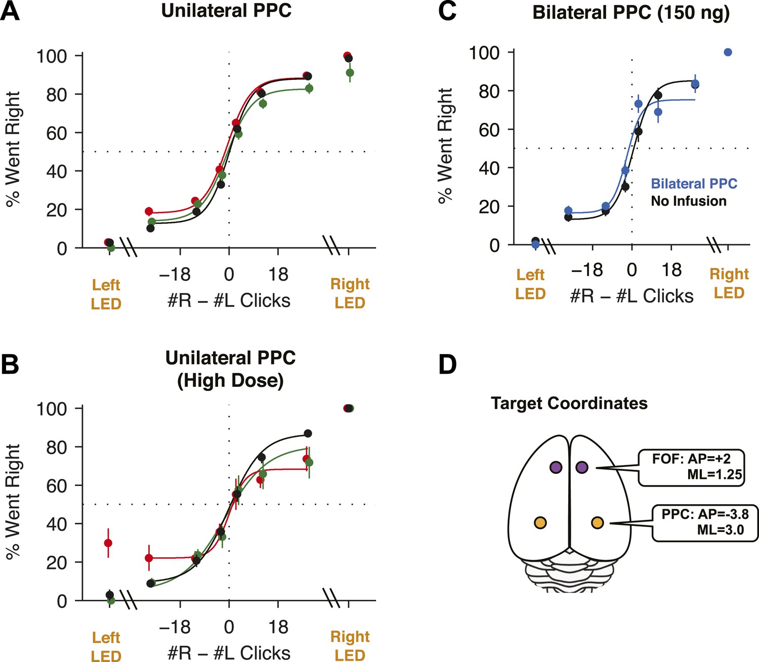
PPC Infusions.
(A) As in Figure 3B, but for unilateral infusions of muscimol into the PPC, which result in a minimal impairment. In black are data from control sessions 1 day before an infusion (n = 65 sessions, 14 rats). In red are data from right PPC infusions (n = 31 sessions, 14 rats, 150 or 300 ng). In green are data from left PPC infusions (n = 34 sessions, 14 rats, 150 or 300 ng). (B) As in (A), but using very high doses of muscimol. Only very small effects are seen. In black are data from control sessions 1 day before an infusion (n = 11 sessions, 9 rats). In red are data from right PPC infusions (n = 3 sessions, 3 rats, 600 or 2500 ng muscimol). In green are data from left PPC infusions (n = 8 sessions, 8 rats, 600 or 2500 ng). (C) Bilateral infusion of muscimol into the PPC does not produce a markedly bigger impairment. In black are data from control sessions 1 day before an infusion (n = 8 sessions, 4 rats). In blue are data from bilateral PPC infusions (n = 8 sessions, 4 rats, 150 ng per side). (D) Schematic view of the brain, duplicated from Figure 3A to remind readers of the location of FOF and PPC on the cortical surface.
Figure 7—figure supplement 1
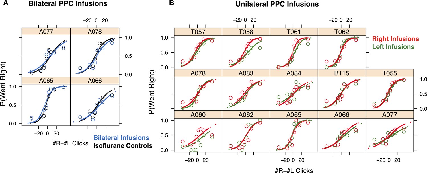
PPC infusions have nominal effects on the Poisson Clicks task.
(A) The psychometric data for accumulation trials and GLMM model fits for bilateral PPC infusions in each rat (n = 4). Open circles are binned data and the small points are the predictions of the GLMM fits at sampled data points. (A) In black are the isoflurane control data and fits and in blue are the bilateral infusion data and fits. (B) The psychometric data and GLMM model fits for unilateral PPC infusions in each rat (n = 14). Open circles are binned data and the small points are the generated by the GLMM fits at sampled data points. In red are the right infusion data and fits and in green are the left infusion data and fits. The difference between right and left infusions is markedly smaller in the PPC than in the FOF.
Figure 8
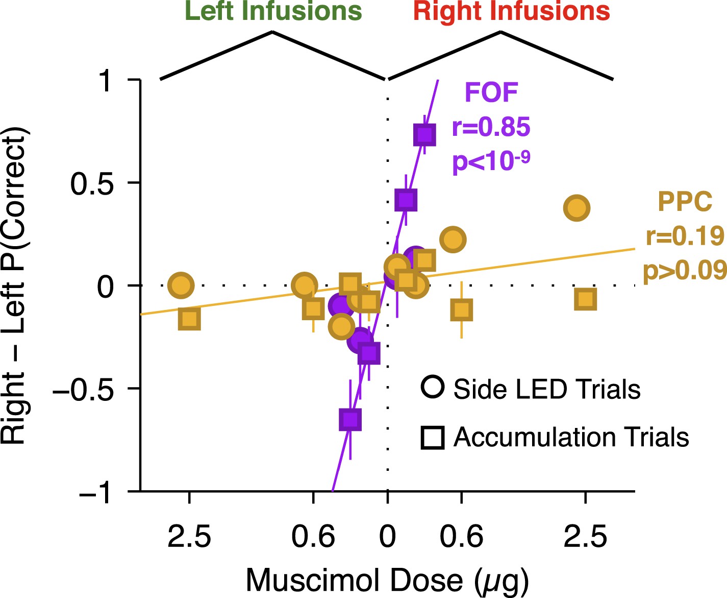
Summary of dose-bias relationship for all unilateral infusions.
Infusions into the FOF are in magenta and into the PPC are in yellow. Circles indicate bias on LED trials, squares indicate bias on accumulation trials. The magenta line is the linear fit between signed dose of FOF infusion (+for right infusions, −for left infusions) and performance bias (right − left % correct) on accumulation trials (r = 0.85, p < 10−9). The yellow line is the linear fit between signed dose of PPC infusion and performance bias on accumulation trials (r = 0.19, p > 0.05). The plotted x-location of the side LED trials are slightly offset for visualization.
Figure 9 with 1 supplement

Unilateral PPC inactivations induce a strong ipsilateral bias during internally guided decisions, and can induce a strong bias on accumulation trials if the FOF is bilaterally inactivated.
(A–D) Effect of unilateral PPC or FOF inactivations on free choice trials intermixed with regular accumulation trials. (A) A schematic of the three interleaved trial types: Accumulation, Side LED and Free Choice trials. Accumulation and side LED trials proceeded as described in Figure 1. On free choice trials (25% of all trials), after withdrawal from the center port both side LEDs were illuminated and rats were rewarded for going to either port. (B) After a few sessions, rats quickly developed an intrinsic bias on free choice trials even while showing no bias on instructed trials (Accumulation and side LED trials). When muscimol was infused into the PPC free choices were significantly biased toward the side of the infusion. This panel shows an example from a single infusion day where the side of the infusions was chosen to be opposite to their intrinsic free-choice bias, together with data from the previous and subsequent control day. (C) Unilateral PPC infusions generated a significant 26 ± 9% (mean ± s.e. across rats, n = 7) ipsilateral bias on free choice trials compared to control sessions (the day earlier). During infusion sessions there was a small 8 ± 4% (mean ± s.e., n = 7 rats) contralateral bias on accumulation trials, perhaps compensatory to the free choice ipsilateral bias. There was no effect on side LED trials (D). Unilateral FOF infusions generated significant ipsilateral biases on free choice and accumulation trials, but not on side LED trials. One rat (A077) was extremely biased (90% Ipsilateral choices) on Side LED trials during FOF inactivation, indicated as an outlier. *p < 0.01. (n = 25 session, 7 rats) (E) Combined bilateral infusion of muscimol into the FOF with unilateral infusion of muscimol into the PPC results in a substantial ipsilateral bias on accumulation trials. In black are data from control sessions 1 day before an infusion (n = 32 sessions, 4 rats). In red are data from bilateral FOF infusions with right PPC infusion (n = 8 sessions, 4 rats, 75 ng per side in the FOF, 300 ng in right PPC). In green are data from bilateral FOF infusions with left PPC infusion (n = 8 sessions, 4 rats, 75 ng per side in the FOF, 300 ng in left PPC). See Figure 9—figure supplement 1 for the individual rat results and GLMM fits.
Figure 9—figure supplement 1
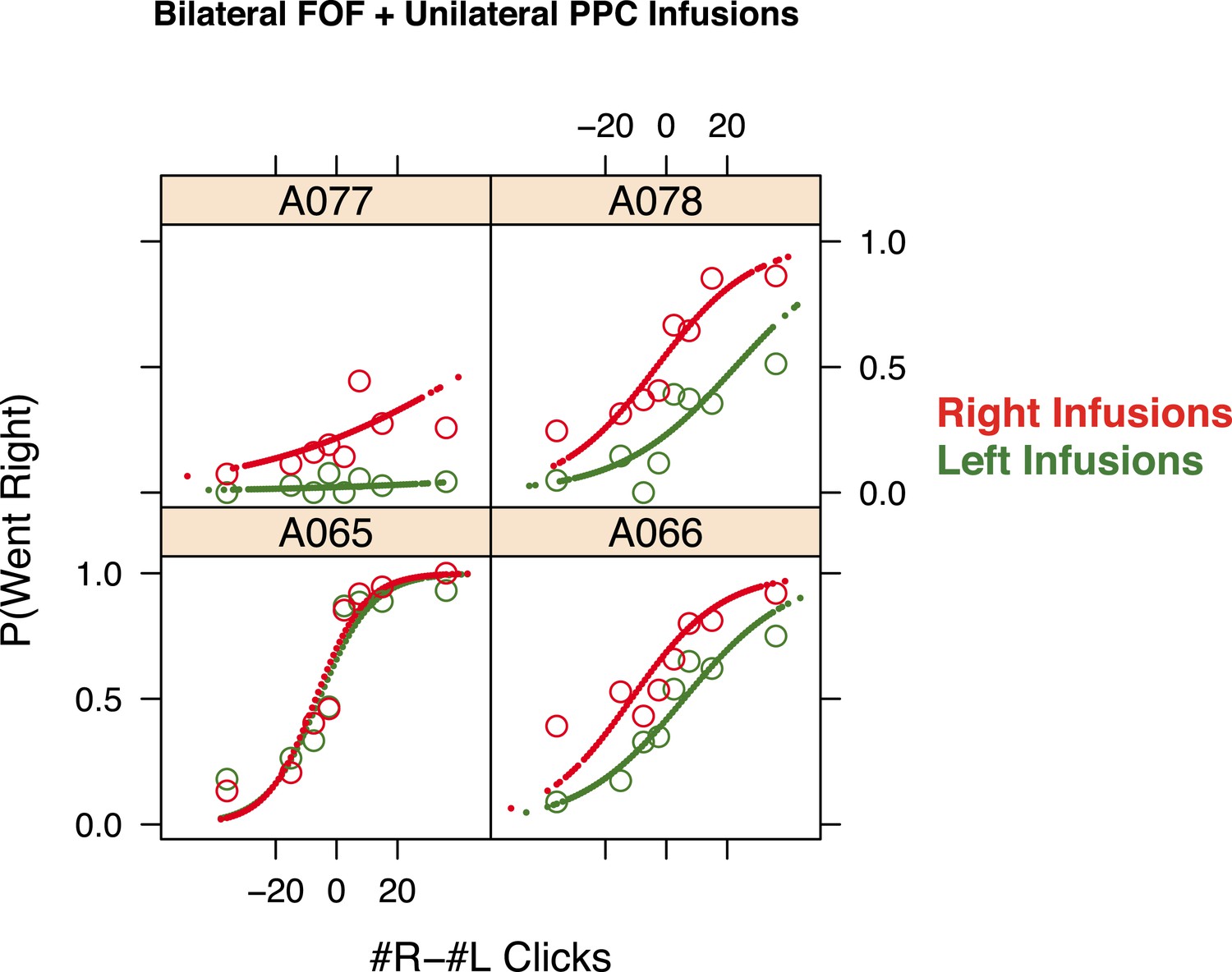
Simultaneous infusion data for each rat.
The psychometric data for accumulation trials and GLMM model fits for bilateral FOF infusions in each rat (n = 4). Open circles are binned data and the small points are the predictions of the GLMM fits at sampled data points. In red are the bilateral FOF + right PPC infusion data and fits and in green are the bilateral FOF + left PPC infusion data and fits. In three of four rats the right infusions lead to significantly more rightward responses than left infusions. There is substantial variability in the overall bias of individual rats in this experiment likely due to the difficulty of performing a perfectly balanced bilateral inactivation of FOF. However, the contribution of the PPC infusion was reliable (3/4 rats) despite an underlying bias.
Tables
Table 1
Best-fit parameters
| Ratname | λ | B | ϕ | τϕ | Þ | lapse | |||
|---|---|---|---|---|---|---|---|---|---|
| B115 | 1.409 | 0.113 | 102.130 | 0.523 | 14.849 | 0.175 | 0.064 | 0.157 | 0.094 |
| T055 | 1.226 | 0.001 | 11.248 | 0.043 | 16.014 | 0.253 | 0.351 | 0.118 | 0.078 |
| T057 | 0.810 | 0.031 | 74.478 | 0.027 | 15.060 | 0.156 | 0.093 | 0.020 | 0.075 |
| T058 | 1.087 | 0.000 | 17.612 | 0.000 | 15.875 | 0.025 | 0.276 | −0.122 | 0.051 |
| T061 | 0.620 | 0.000 | 96.545 | 0.502 | 16.038 | 0.380 | 0.041 | 0.236 | 0.066 |
| T062 | −0.098 | 0.000 | 49.361 | 0.619 | 15.761 | 0.139 | 0.047 | 0.518 | 0.083 |
| A065 | 2.047 | 0.000 | 37.685 | 0.207 | 15.729 | 0.147 | 0.092 | −0.465 | 0.031 |
| A066 | 0.349 | 0.000 | 15.565 | 0.000 | 12.705 | 0.072 | 0.462 | 0.041 | 0.170 |
| A077 | −2.739 | 0.197 | 128.586 | 22.801 | 9.253 | 0.184 | 0.031 | 0.886 | 0.001 |
| A078 | −2.070 | 0.000 | 104.688 | 0.000 | 18.086 | 0.283 | 0.026 | 0.062 | 0.063 |
| A060 | −1.542 | 0.000 | 54.786 | 0.000 | 15.416 | 0.010 | 0.115 | 0.180 | 0.245 |
| A062 | 2.258 | 0.296 | 156.860 | 0.486 | 16.839 | 0.527 | 0.076 | 0.466 | 0.119 |
| A083 | −0.790 | 47.441 | 31.788 | 1.384 | 16.282 | 0.015 | 0.059 | 0.033 | 0.107 |
| A084 | 1.371 | 0.064 | 70.267 | 1.690 | 15.011 | 0.016 | 0.086 | 0.467 | 0.110 |
| Meta-Rat | 1.227 | 0.001 | 57.614 | 0.043 | 16.042 | 0.221 | 0.109 | 0.065 | 0.102 |
| BiFOF | −4.144* | 62.423 | 237.642 | 1.754 | 22.013 | 0.082 | 0.039 | 0.737* | 0.010 |
| BiPPC | 1.331 | 0.531 | 42.175 | 0.000 | 14.860 | 0.512 | 0.175 | −0.249 | 0.321 |
-
This table shows the values of the parameters which maximize the likelihood of the full 9-parameter accumulator model for each rat, as well as for the ‘meta-rat’ (made from taking all of the control days that were 1 day before an infusion, n = 47,580 trials), the fit to the bilateral FOF data (n = 1809), and the fit to the bilateral PPC data (n = 1569).
-
*
indicate parameters that were significantly different from the control ‘Meta-Rat’.
Table 2
Bilateral FOF model comparison
| Model | # of param. | Log likelihood | BIC | AIC |
|---|---|---|---|---|
| full model | 9 | −1102.5 | 2272.5 | 2223† |
| Þ model | 1 | −1221.6 | 2450.7 | 2445.2 |
| λ model | 1 | −1121.1 | 2249.7* | 2244.2 |
-
This table shows the three models fit to the bilateral FOF data (n = 1809 trials).
-
*
indicates the model with the lowest (the most likely) Bayesian information criterion (BIC).
-
†
indicates the model with the lowest (most informative) Akaike information criterion (AIC).
-
In this case, the AIC and BIC select different models, suggesting a better model may be somewhere in between. That is, a model that includes the accumulator time-constant and perhaps a few additional parameters from the full model.
Table 3
Unilateral FOF model comparison
| Model | # of parameters | Log likelihood | BIC | AIC |
|---|---|---|---|---|
| Post-categorization bias | 1 | −1963.1 | 3934.4* | 3928.2† |
| Unbalanced input gain | 1 | −2013.1 | 4034.4 | 4028.2 |
| Accumulator shift | 1 | −2217.4 | 4443.0 | 4436.8 |
| Unbalanced input noise | 1 | −2272.7 | 4553.7 | 4547.4 |
| 8-parameter model | 8 | −1957.5 | 3981.1 | 3949.9 |
-
This table shows the three models fit to the unilateral FOF data (n = 3836 trials).
-
*
indicates the model with the lowest Bayesian information criteria (BIC), that is, the most likely model.
-
†
indicates the model with the lowest Akaike information criteria (AIC), that is, the most informative model.
-
The 1-parameter post-categorization model has the lowest AIC and BIC, supporting the view that the major effect of unilateral FOF inactivation is not related to the accumulation process per se.
Additional files
-
Supplementary file 1
Using the lme4 package to fit generalized-liner mixed models in R. This file contains the code (and links to our data) which shows how we used the lme4 package, in R, to fit generalized linear mixed models (GLMM). We also include the output of each of the GLMM we described in the main text. This allows the interested reader to regenerate our main results and also, by providing the data, allows the reader to perform additional statistical tests.
- https://doi.org/10.7554/eLife.05457.024
Download links
A two-part list of links to download the article, or parts of the article, in various formats.
Downloads (link to download the article as PDF)
Open citations (links to open the citations from this article in various online reference manager services)
Cite this article (links to download the citations from this article in formats compatible with various reference manager tools)
Distinct effects of prefrontal and parietal cortex inactivations on an accumulation of evidence task in the rat
eLife 4:e05457.
https://doi.org/10.7554/eLife.05457


