A thesaurus for a neural population code
- Weizmann Institute of Science, Israel
- Ben-Gurion University of the Negev, Israel
Figures
Figure 1
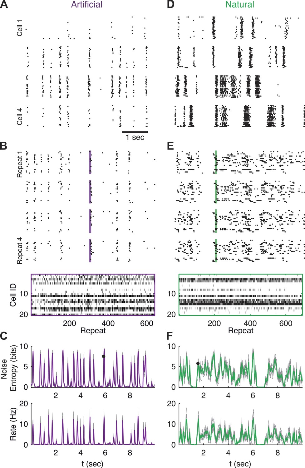
Population responses to natural and artificial stimuli are noisy.
(A) Subset of the responses of four retinal ganglion cells to 20 repeats of the same artificial video clip (out of 641 altogether). Each block corresponds to one cell, each line to a single repeat; black dots mark spike times. (B) Top: Response of a population of 20 retinal ganglion cells to four repeats of the same stimulus as in A. Here, each block represents the response of the entire population in a single trial and each line represents a single cell. Bottom: All 641 population responses of the 20 cells (across repeats) for one time point marked by the shaded bar in the raster plot above. Black ticks represent spikes; each vertical slice in the plot is the population response on a single trial and is therefore a single sample from the conditional distribution of responses given the stimulus presented at that point in time P(r|s). (C) Top: Conditional entropy of the population response patterns, given the stimulus, as a function of time for a 10 s artificial video clip repeated hundreds of times. Thin gray lines correspond to different groups of 20 cells; Average over 10 groups is shown in purple. Bottom: The average firing rate, for the same stimulus, shown as a function of time. (D–F) Same as A–C but for a natural video clip (with 693 repeats).
Figure 2 with 2 supplements

Strong noise correlations, at the population level, at interesting times in the video.
(A) Population noise correlation, measured by the multi-information over the conditional population responses, at each point in time in response to an artificial video. Thin gray lines correspond to individual groups of 20 cells; average over groups is shown in purple. (B) Population noise correlation as a function of average population firing rate for one representative group. Interesting events in the video evoke a vigorous response by the retina, characterized by strong network correlations. (C) Distribution of spike counts across different repeats of the same stimulus for the time point marked by black dot in A. Purple dots correspond to empirical estimates, gray line is what we would expect if neurons were conditionally independent, given the stimulus; and red line is the prediction of the maximum entropy pairwise model. (D–F) Same as A–C but for a natural video clip.
Figure 2—figure supplement 1
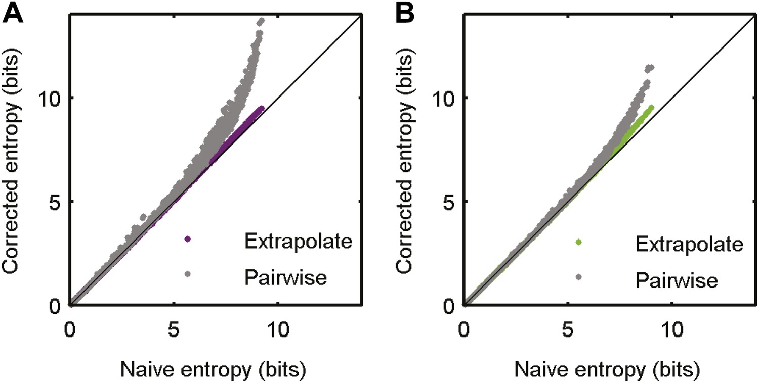
Accurate sampling of entropy.
(A) Pairwise maximum entropy upper bound on entropy (gray) and the extrapolation corrected noise entropy (Treves and Panzeri, 1995; Strong et al., 1998) (purple) are shown as a function of the naive noise entropy estimate. Each dot corresponds to the distribution at a single time point in the artificial video; black line marks identity. The bias corrections are on the order of a few percent at most. (B) Same as A, but for data taken from the natural video data set (693 repeats).
Figure 2—figure supplement 2
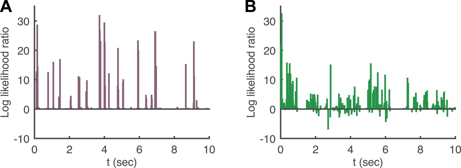
Log likelihood ratio of the pairwise model and the conditionally independent model.
(A) A pairwise (second order maximum entropy as in the text) and an independent model (product of marginals) was fit to each time point (equivalently stimulus) in the artificial video using 90% of video repeats. The log likelihood ratio of the two models (log[LikelihoodPairwise/LikelihoodCond. − Indep.]) is plotted as a function of time (equivalently stimulus), for the held out 10% of repeats. The likelihoods are similar much of the time, corresponding to low firing epochs, but for many points in time the likelihood of the pairwise model can be orders of magnitude higher. (B) Same as A, for the natural video.
Figure 3 with 2 supplements
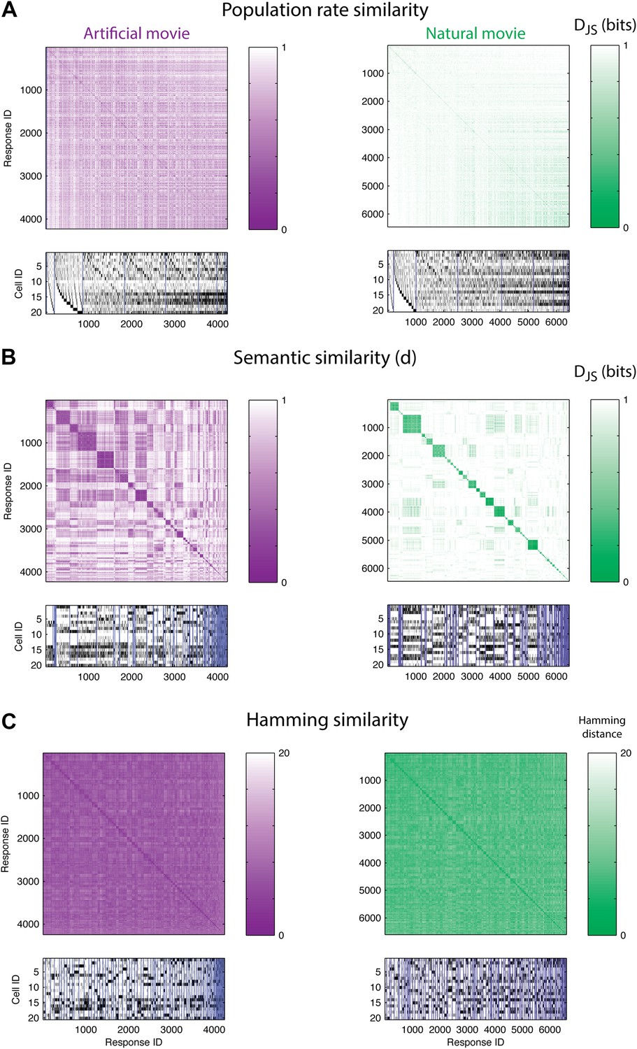
The population code of the retina is comprised of clusters of responses with highly similar meaning.
(A) Top: Similarity matrices of the population responses of representative groups of 20 neurons to an artificial (left) and natural (right) video. Each entry in the matrix corresponds to the similarity, d (see text), between two population responses observed in the test data (responses shown at bottom). Matrix rows (and columns) are ordered by total spike count in the population responses. Bottom: The population responses corresponding to the entries in the matrix; black ticks represent spikes. Each column is a population activity pattern corresponding to the matrix column directly above. Blue lines mark borders between different clusters. The lack of structure in the matrices implies that population responses with similar spike counts do not carry similar meanings. (B) Same as A, only here the matrix is clustered into 120 clusters. Matrix rows (and columns) are ordered such that responses from the same cluster appear together. A clustered organization of the population code is clearly evident. (C) Same as B, but using the Hamming distance between population responses, instead of the similarity measure d. A simple measure of syntactic similarity does not reveal the underlying clustered organization of the code.
Figure 3—figure supplement 1
Clustered organization is highly significant.
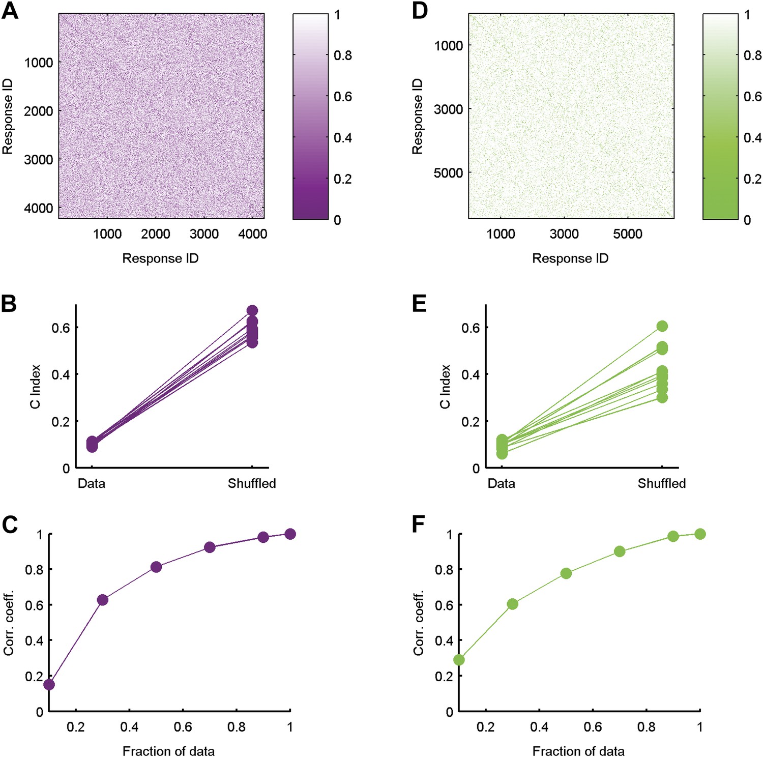
(A) The similarity matrix used in Figure 3 in the main text was first randomly shuffled and only then clustered. Clearly the grouping structure has disappeared, suggesting the structure is a property of the code's organization and not the values in the matrix or the power of the clustering algorithm. (B) For each of the ten 20 neuron groups we calculated the C Index (Hubert and Schultz, 2011) (left, labeled ‘Data’), which measures goodness of clustering; a smaller C Index corresponds to better clustering. For each matrix, we then measured the C Index for 100 randomly shuffled versions and took the minimal value of all shuffled matrices (right, labeled ‘Shuffled’). None of the shuffled values came close to the real values, indicating a p-value smaller than 0.01 for each matrix. (C) Correlation coefficient between similarity matrices estimated using different fractions of data. Overall we had 641 repeats of the artificial video. Using 70% of the repeats, we are at ∼0.9 correlation with our estimates using all available repeats (Data are for the same matrix shown in Figure 3 of main text). (D–F) Same as A–C but for data taken from the natural video data set.
Figure 3—figure supplement 2
Semantic similarity between population patterns can be explained by a simple local similarity measure, but not by a global similarity measure.
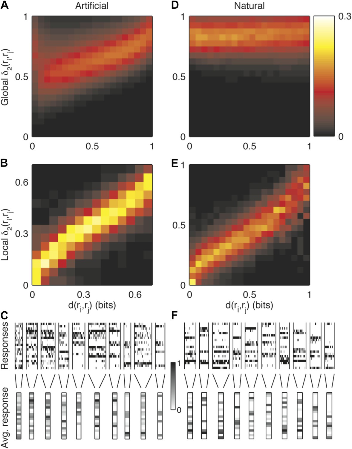
(A) We sought a simple formula to approximate the similarity measure d, in the spirit of the measures described in Victor and Purpura (1997); van Rossum (2001); Houghton and Sen (2008). The Hamming distance gave a very poor approximation of similarity and even a measure which gave a different weight to each neuron, , performed very poorly. Shown is a joint histogram of the similarity values d(ri,rj) (x-axis) and the corresponding values predicted by a global second order similarity model (y-axis. w parameters fit to train data; results for cross-validated test data are shown) for the responses of a representative group of 20 neurons (same as in Figure 3) to an artificial video. For clarity, values were normalized about the y-axis, such that each vertical slice sums to one. (B) Joint histogram of the similarity values of pairs of responses from the same cluster (x-axis) and the similarity predicted by a local second order model for similarity, that is, δ2 applied independently to each cluster. Other details as in A. These results suggest that noise is highly stimulus dependent and cannot be accurately described by a global, stimulus independent, model. Yet, for a given cluster, we can accurately describe its similarity neighborhood, using the appropriate set of single neurons and neuron pairs. (C) In support of the previous conclusion, we found that close inspection of large response clusters reveals an obvious structure within clusters. Many of the clusters of similar responses can be characterized as having very precise neurons (almost always spiking or almost always silent), alongside more noisy neurons, which appear to be nearly random within a cluster. These precise and noisy neurons differ from one cluster to another. Shown is a detailed view of the responses in a subset of the clusters, which contain between 20 and 50 different patterns and appear most frequently in the data. Top: All population responses belonging to each cluster (clusters separated by vertical lines). Each horizontal line corresponds to one neuron; each vertical slice is the response of the population to a single repeat. Bottom: The average response of each cluster. The spiking probability of each neuron is represented by its gray scale intensity (color bar: dark—high spike probability, light—low spike probability). (D-F) same as (A-C), but for a natural video stimulus.
Figure 4 with 1 supplement
Responses to the same stimulus tend to come from the same cluster.
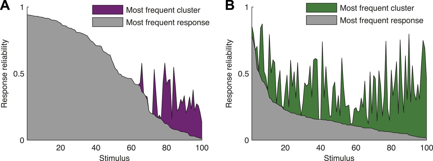
(A) The probability of the most frequent response across video repeats is plotted as a function of stimulus identity in gray (stimuli are sorted by reliability). In purple, we plot the reliability of the clustered response, that is, the probability of observing a response from the most frequent cluster for each stimulus (clustering matrix presented in Figure 3). Only the 100 stimuli that evoked the strongest response are shown. Clearly, responses to the same stimulus tend to come from the same cluster, even when the most frequent single response occurs less than 20% of the time, thus the cluster code is far less noisy. (B) Same as A but for the natural video data set.
Figure 4—figure supplement 1

Increased reliability of clustered responses is highly significant.
(A) Responses recorded at the same time point across video repeats cluster together significantly. Shown is the probability of the most frequent cluster, plotted as a function of stimulus id (purple; stimuli sorted by reliability), for the clustered response; that is, the probability of the most frequent cluster evoked by each stimulus (same as Figure 4A). For comparison, we also shuffled the cluster assignment of each response and repeated the analysis. Shown in gray is mean ± STD of the most frequent cluster in 100 randomly shuffled cluster assignments. Clearly, for many time points the high reliability of the clustered response is not merely a result of response grouping, but the tendency of responses from the same cluster to be associated with the same stimulus. (B) Same as A, but for natural video data set.
Figure 5 with 4 supplements
Cluster identity conveys most of the information about the stimulus.
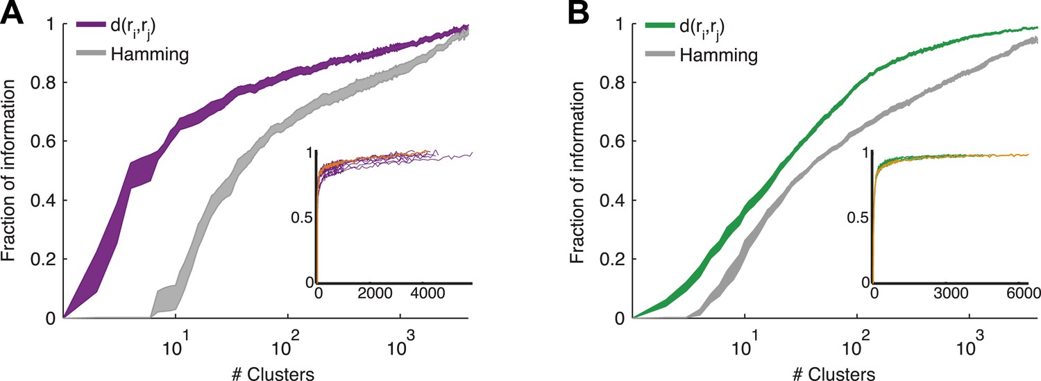
(A) The fraction of information retained about the stimulus when population responses are replaced with the label of the cluster they belong to, plotted as a function of the number of clusters used. Lines correspond to the average of 10 groups of 20 neurons, line widths represent SEM. Purple—clustering based on the similarity measure described in the text, gray—clustering based on the Hamming distance. Inset: Fraction of information as a function of the number of clusters on a linear scale. Individual groups are shown in gray, and the orange line marks the curve corresponding to the representative matrix from Figure 3. Very few clusters are required to account for most of the information, suggesting responses from the same cluster have a similar meaning. (B) Same as A, but for a natural video clip.
Figure 5—figure supplement 1
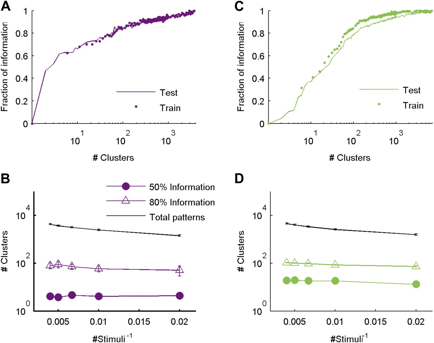
The similarity measure generalizes well across stimuli.
(A) Fraction of information retained about the stimulus plotted against the number of response clusters. The similarity measure learned from the artificial video train data is applied either to cross-validated test data (same as Figure 5 of main text; purple line), or to the train data itself (purple dots). We see nearly identical performance on cross-validated and non cross-validated data. Shown is the same representative group of 20 neurons as in Figure 3. (B) The number of clusters required to recover over 50% (filled purple circles) or 80% (open triangles) of the information available about the stimulus, plotted as a function of the inverse number of stimuli in the test data (train data remained fixed), on a semi-logarithmic scale. Also shown, for comparison, is the overall number of observed patterns (black line). Depicted are average and SEM (may be smaller than markers) over 10 different groups of 20 neurons. As the number of stimuli in the test set increased, we saw a very mild increase in the number of clusters required to account for either 50% or 80% of the information. In fact, there was no significant increase in the number of clusters when the number of stimuli increased from 200 to 250 (p > 0.4, sign rank test), while the number of observed patterns grew significantly by over 500 (p < 0.01 sign rank test). This suggests that the clusters (or ‘code-words’) we identified are relevant to a wide range of stimuli within the same stimulus class. (C, D) Same as panels A and B, but for data taken from the natural video data set.
Figure 5—figure supplement 2

Clustering aimed at maximizing the mutual information yields similar results to clustering based on similarity alone.
(A) Fraction of information retained about the stimulus plotted against the number of response clusters (full field flicker stimulus). Responses were either clustered using simple agglomerative clustering (purple. Same as in main text, see ‘Materials and methods’), or using agglomerative information bottleneck clustering (Slonim and Tishby, 1999), which explicitly aims to cluster responses such that maximal information about the stimulus is retained (black). Although, we would expect clustering aimed at information maximization to do a better job, after cross-validation (applying the clustering to novel responses to novel stimuli), we see that the simple similarity based clustering performs just as well. The data shown are for the same representative group as used throughout the main text. We note that results are shown for cross-validated test data, and that information bottleneck clustering is a greedy approach with no guarantee of optimality, thus it is possible for similarity based clustering to outperform information bottleneck clustering. (B) Same as A, but for the responses to a natural video stimulus.
Figure 5—figure supplement 3
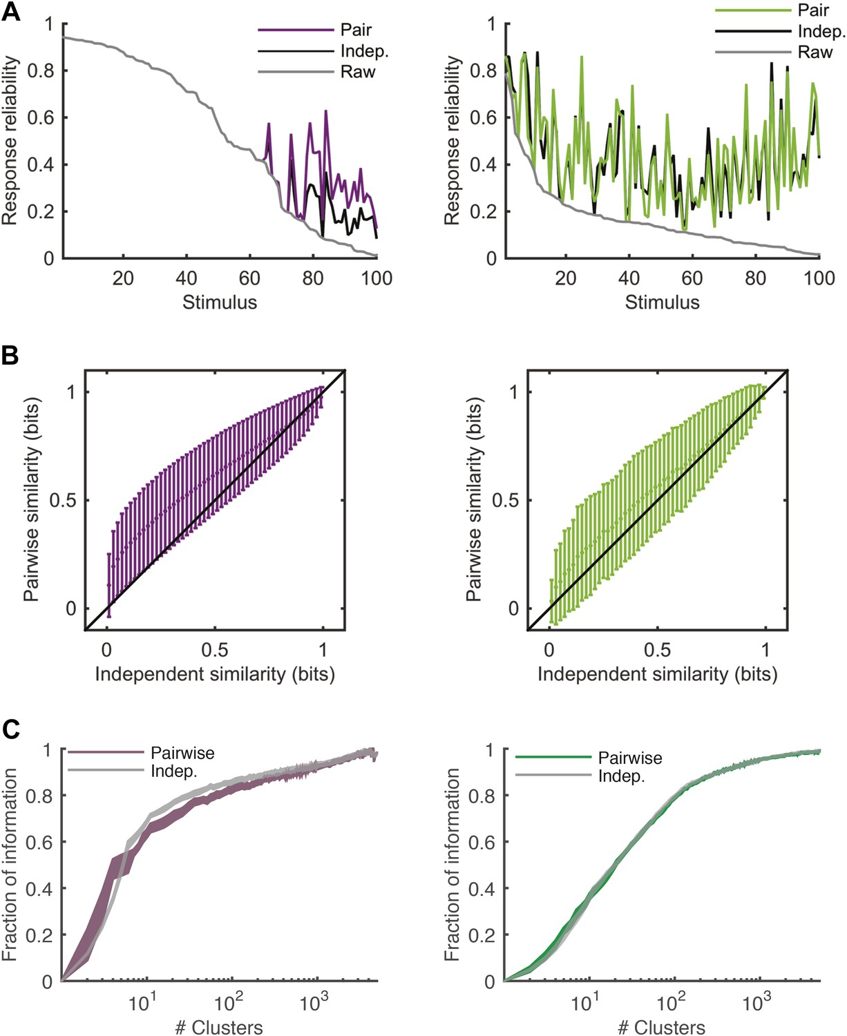
Comparing response similarity derived from the conditionally independent model and pairwise model.
(A) Left: The probability of observing the most frequent response across repeats of the artificial video is plotted as a function of stimulus i.d. in gray; for clarity, the stimuli are sorted by reliability of their responses. In black is the reliability of the clustered response, that is, the probability of the most frequent cluster evoked by each stimulus, where responses were clustered by similarity derived from a conditionally independent model. In purple is the clustered reliability as derived from the pairwise model used in the main text (same as Figure 4). Only stimuli that evoked a strong response (at least one spike in over 75% of the repeats) are shown. Here, reliability is much higher when using the more accurate pairwise model to derive similarity between population responses. Right: Same as left, but for the Natural video data set. Here, differences between conditionally independent and pairwise models are less pronounced. (B) Left: Similarity derived from the conditionally independent model is directly compared with the similarity derived from the pairwise model, for test responses to the artificial video. Similarities between response pairs calculated using the conditionally independent model were binned (x-axis) and the mean and standard deviation of the similarity for the same pairs was calculated using the pairwise model (y-axis). Black line marks identity. Right: Same as left, but for the natural video. We see that similarity measured using the conditionally independent model is closer to that measured using the more accurate pairwise model under natural stimulation. (C) Left: same as Figure 5A, but here we compare the fraction of information as a function of number of clusters curve obtained by using the pairwise model (purple) and the one obtained using the conditionally independent model, in which noise correlations are ignored (gray).
Figure 5—figure supplement 4
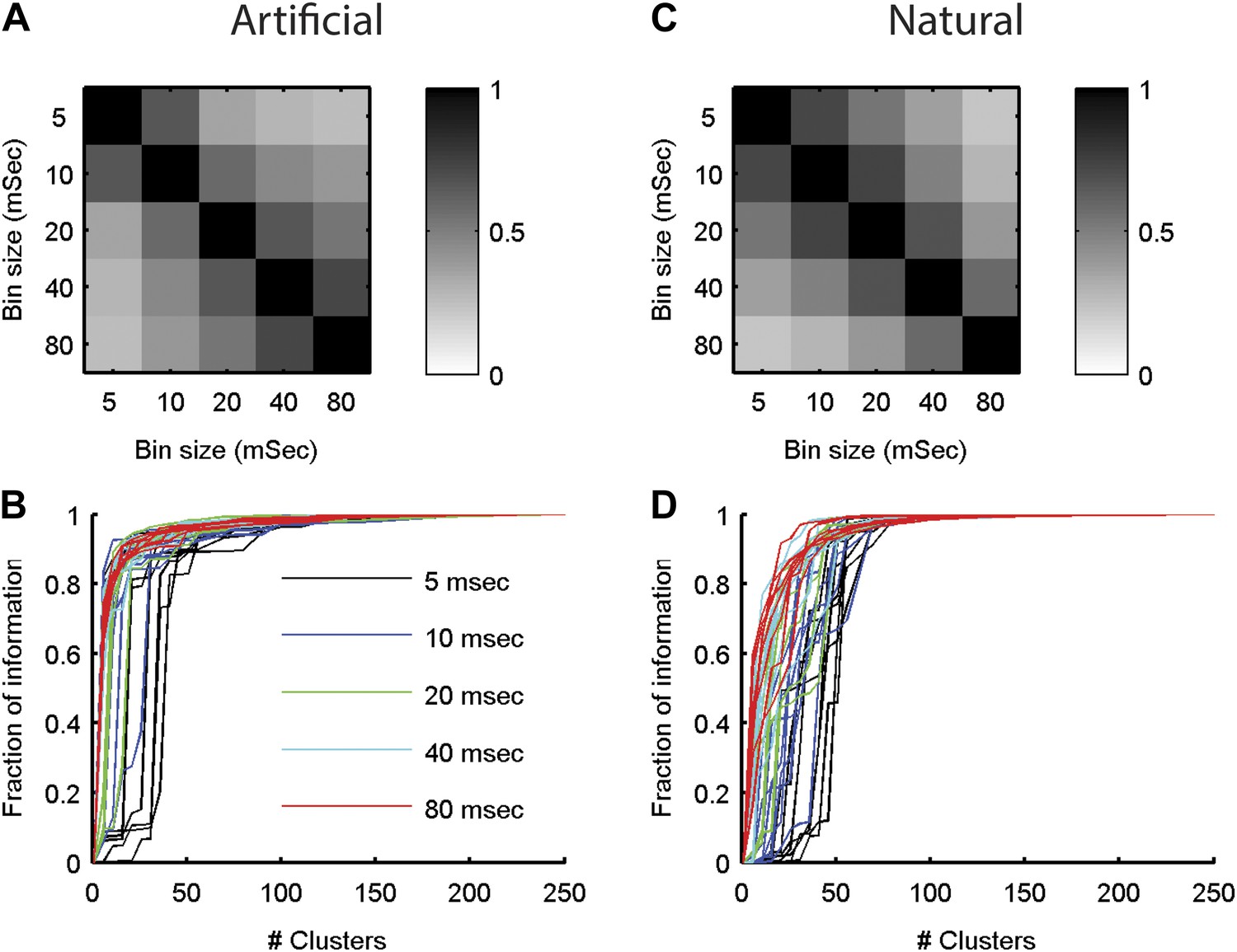
The neural ‘thesaurus’ remains stable across different bin sizes.
(A) Correlation matrix between the similarity values estimated for all possible response pairs. For a given group of 8 neurons from the artificial video data set, we calculated the full similarity matrix over all 256 possible responses. This was done for bin sizes between 5 and 80 ms. We then calculated the correlation between the similarity matrices for each combination of bin sizes. Shown is an average across 8 randomly chosen groups of 8 neurons. The results indicate that except for extreme differences in bin size, we recover highly consistent similarity structures. (B) The fraction of information is shown as a function of the number of clusters in the similarity matrix (compare to Figure 5 in main text). Different bin sizes are indicated by colors. Different lines correspond to different individual 8 neuron groups (same groups as A). We see very similar results except for the very short time bin of 5 ms. (C, D) Same as A and B but for data taken from the natural video data set.
Figure 6 with 1 supplement
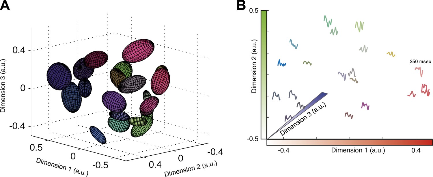
Response similarity predicts stimulus similarity.
(A) The responses belonging to clusters that contain 30–300 patterns were embedded using Isomap. Each ellipse represents the 1 STD Gaussian fit to all responses belonging to a single cluster. The Euclidean distance in the plot approximates the similarity measure d (see text). The coordinates also correspond to the RGB value of each ellipse, thus nearby clusters share similar colors. Same representative group as in Figure 3. (B) Embedding of cluster triggered average waveforms in 2D Euclidean space. For each pair of clusters from panel A, we calculated the inter-cluster distance as the average similarity between pairs of responses, one from each cluster. Clusters were then embedded in 2D space using Isomap in a manner that approximates the calculated distances. Each cluster is represented by the mean stimulus that preceded (250 ms) responses belonging to that cluster. Thus, nearby waveforms belong to similar clusters. Clusters are colored as in panel A, therefore the blue channel corresponds to the third dimension of embedding not shown in the plot.
Figure 6—figure supplement 1
Cluster similarity implies stimulus similarity.
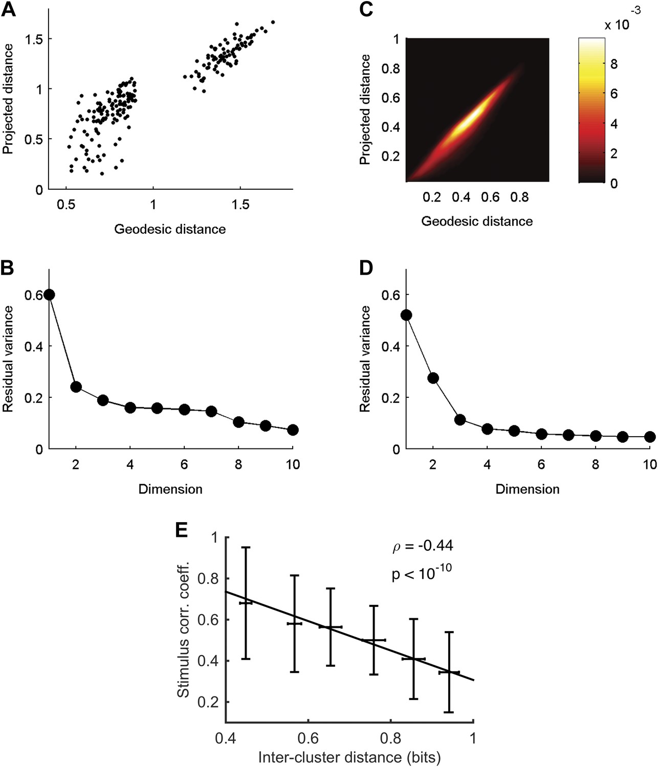
(A) Geodesic vs embedded distances for the embedding shown in Figure 6A. The x-axis is the Geodesic distance between clusters (i.e., distances in the neighborhood graph; methods), vs the Euclidean distances after embedding in 3D. (B) Residual variance as a function of dimensionality for embedding of waveforms in Figure 6A. The residual variance is defined as 1 − r2(dG,dIso), where r is the correlation coefficient, dG is the geodesic distances between points as defined by the weighted neighborhood graph (Tenenbaum et al., 2000), and dIso is the Euclidean distances between points after embedding. (C) Same as A, but for embedding of responses in Figure 6B. Due to the large number of population responses embedded (2391), we show the joint histogram of the geodesic (x-axis) and embedded (y-axis) distance values. Colorbar represents frequency of occurrence of distance pairs. (D) Same as B, but for embedding of responses in Figure 6B. (E) For each pair of clusters shown in Figure 6A, we calculated the correlation coefficient between the cluster triggered average stimulus (the average of all stimuli preceding responses in a cluster) of each cluster, and plot it as a function of the distance between the clusters. Inter cluster distance was defined as the average similarity between pairs of responses, one from each cluster. Even though the correlation coefficient is not the ideal measure to quantify similarity among stimuli, we still see a clear and significant relationship between cluster similarity and stimulus similarity. Namely, clusters that are more similar (smaller values on the x-axis) have a higher correlation between their associated average stimuli.
Figure 7 with 1 supplement
Accurate decoding of new stimuli from previously unseen population responses, using a neural thesaurus.
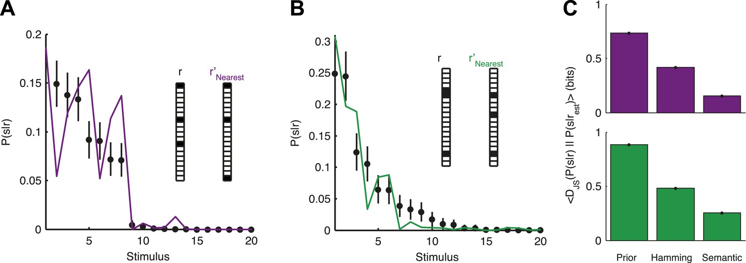
(A) The conditional distribution over stimuli for one population response, P(s|r), to the artificial video is shown (black dots). P(s|r) can be well approximated by the conditional distribution over stimuli P(s|r′) where r′ is the response most similar to r according to the thesaurus d (‘r′Nearest’, purple line). Actual responses are shown as inset. The same representative group of 20 neurons shown in Figure 3 was used here. Error bars represent standard errors of the probability estimates B. Same as in A, but for a natural video clip. (C) Top: The average Jensen-Shannon divergence between the ‘true’ P(s|r) and the estimate described in panel A (Semantic), or for an estimate derived using the Hamming distance instead of our similarity measure (Hamming), for the artificial video data. Also shown is the average divergence from the prior over stimuli (Prior). Plotted are mean and standard errors (barely discernable) across all patterns that had at least one close neighbor (<0.25 bits away). Bottom: Same as above, but for the natural video data. Having a thesaurus markedly improves our ability to gain some knowledge about never before seen responses, compared to a naive prior, or even to using Hamming distance as a similarity measure.
Figure 7—figure supplement 1
Comparing decoding performance using the conditionally independent model and pairwise model.
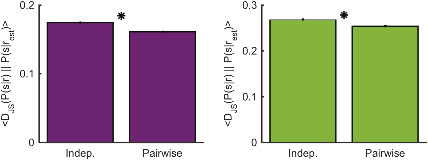
Left: The average Jensen-Shannon divergence between the ‘true’ P(s|r) and the estimate based on the most similar response as measured using either the conditionally independent model or the pairwise model used in the main text (see Figure 7), for responses evoked by an artificial video. Plotted are mean and standard errors (barely discernable) across all patterns that had at least one close neighbor (<0.25 bits away). The pairwise model performs on average slightly yet significantly better (p < 10−4, two-sided paired sign test). Right: Same as left, but for the natural video. Again, the pairwise model performs on average slightly yet significantly better (p < 10−4, two-sided paired sign test).
Videos
Video 1
Embedding of responses in 3D using Isomap.
Each dot represents a single population response to the artificial video; the Euclidean distance between points approximates the similarity d between them. Similar to Figure 6A, only we explicitly plot every population activity pattern in each cluster. Colors represent different clusters and correspond to the colors in Figure 6A,B.
Additional files
-
Source code 1
MATLAB code used in the clustering and information analyses.
This .m file contains functions used in the analyses presented in the paper. It is not intended to be run as is, instead each function needs to be copied and placed in its own .m file. These functions are also available at the following GitHub respository - https://github.com/eladganmor/Neural_Thesaurus
- https://doi.org/10.7554/eLife.06134.022
Download links
A two-part list of links to download the article, or parts of the article, in various formats.
Downloads (link to download the article as PDF)
Open citations (links to open the citations from this article in various online reference manager services)
Cite this article (links to download the citations from this article in formats compatible with various reference manager tools)
A thesaurus for a neural population code
eLife 4:e06134.
https://doi.org/10.7554/eLife.06134


