Female mice ultrasonically interact with males during courtship displays
- Janelia Research Campus, Howard Hughes Medical Institute, United States
- University of Delaware, United States
Figures
Figure 1
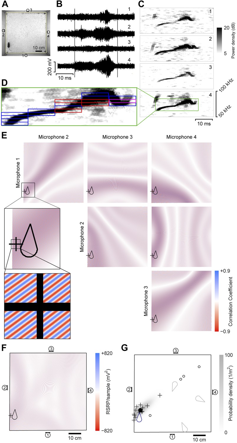
Illustration of sound-source localization procedure.
(A) Image shows the location of a mouse in the behavioral arena during one video frame. Microphone locations are indicated by numbered microphone symbols (a circle with a tangent line segment). Yellow quadrilateral indicates the floor boundaries. (B) Vocal signal recorded at the same time as the frame in panel A. The number of each signal corresponds to the microphone in A. Vertical lines indicate the start and end of the signal extracted by the audio segmentation software. (C) Spectrograms of the signals in B. Numbers in upper-right corner indicate the corresponding microphone. In the fourth microphone spectrogram, the large green rectangle indicates the time- and frequency-bounding box determined by the audio segmentation software. (D) Smaller rectangles indicate the ‘snippets’ calculated from the segment and the associated frequency contour. Small red rectangles indicate snippets that were eventually discarded (see below). Small magenta rectangle is the snippet highlighted in panel E. (E) Correlation coefficient maps determined from each microphone pair. In each map, the color represents the correlation coefficient between the two microphone signals once each is time-shifted appropriately for that position. Thus, deep blue/red points represent likely/unlikely source locations, given the information just in this snippet, for just this microphone pair. Plus symbol (+) represents the source location eventually estimated from this individual snippet (see below). Mouse icon represents mouse location. Inset is an enlargement of the area indicated in the upper left map, to show closely intercalated red and blue bands. Map boundaries correspond to the floor outline indicated in A. (F) Reduced steered response power (RSRP) map for the example snippet. Plus symbol (+) represents the location estimate for this snippet, and corresponds to the highest (positive) value in the map. Black boundary corresponds to the floor outline in A, and microphone locations are indicated by numbered microphone symbols. (G) Consensus estimate from all snippets. Plus symbols (+) and open circles represent single-snippet estimates from all snippets for this segment. Open circles are those snippets determined to be outliers, and non-outlier snippets are pluses. Closed circle indicates the mean of the non-outlier estimates. Gray shading is the probability density of a Gaussian distribution with the mean and covariance matrix of the non-outlier estimates. Mouse probability index value that the vocalization came from the actual mouse was determined to be approximately 1, and from three randomly located virtual mice (gray mouse icons) were 10−11, 10−56, and 10−75. To generate three virtual mouse positions, we picked three random points within the floor of the cage. Black boundary corresponds to the floor outline in A, and microphone locations are indicated by numbered microphone symbols.
Figure 2

Accuracy and precision of sound-source localization system.
(A) Heat map shows inverse relationship between MPI and the distance between the mouse and estimated sound source location (r = -0.66; p < 10-5). The heat map is plotted in log counts with red indicating the maximum. Data for real and virtual mice are included in the plot. (B) Left panel shows the MPI threshold plotted relative to the percent of localized signals that were assigned. Right panel indicates the percentage of accurately assigned vocal signals plotted as a function of MPI threshold. (C) Distribution of the errors between the location of the estimated sound source and real source for assigned vocalizations. Median error is plotted in red. Inset shows the cumulative probability histogram of the errors. (D) Distribution of distances between the mouse assigned the vocalization and the animal closest to the assigned mouse. (E) Heat map showing sound source estimates (n = 2590) relative to mouse position (nose shifted to origin and rotated upwards). Gray sector shows mouse body. The large gray square, which is divided into smaller squares, indicates the regions of interest used to determine the precision of sound source localization system. Yellow key located at the bottom left indicates numbering scheme for smaller regions of interest. (F) Bar plot showing the number of sound source localization estimates in each of the smaller regions of interest. Region 5 includes the head of the mouse. Red line shows the expected counts based on a uniform distribution. The distribution of predicted sound source locations was significantly different between regions ( = 2305.7, p < 10−5).
Figure 3
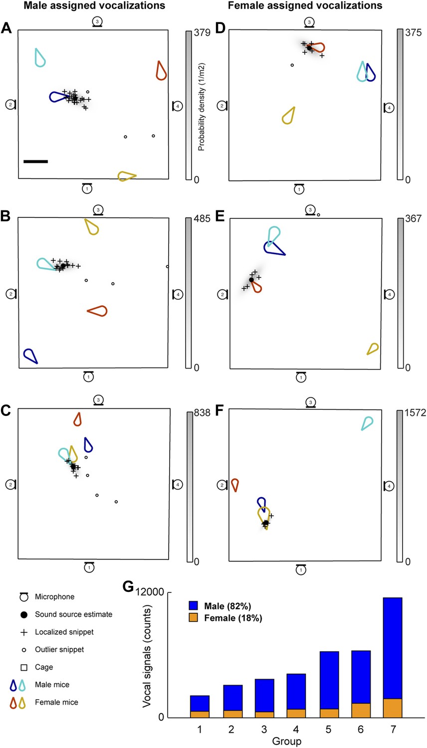
Microphone array reveals both male and female mice vocalize during social interactions.
(A–C) Examples of sound source assigned to a male mice in the presence of multiple mice. (D–F) Examples of sound source assigned to female mice when groups of mice are present. (G) Male (blue) and female (orange) vocal signal counts during each recording session (groups displayed in ascending order of total call number).
Figure 4
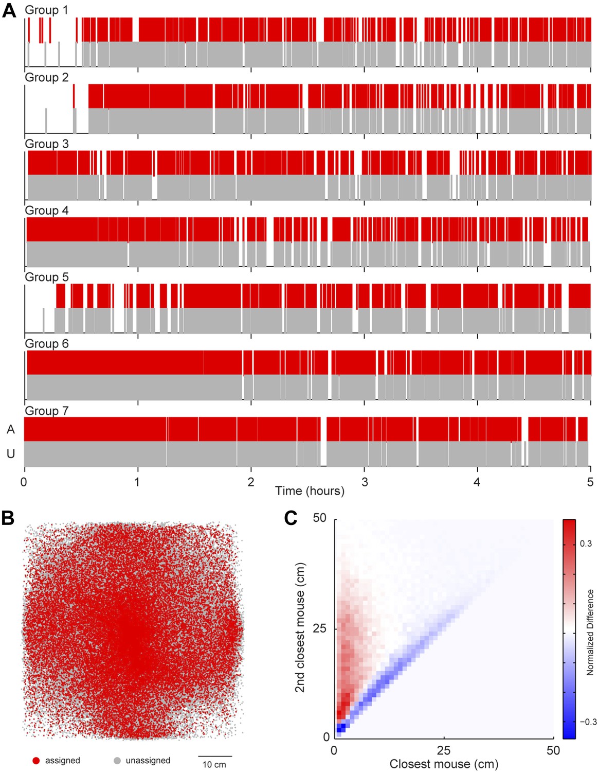
Potential sources of bias in vocalization assignment.
(A) Assigned (red) and unassigned (gray) vocalizations are plotted as a function of time. In all groups, assigned and unassigned vocalizations occur throughout the experiment. (B) The estimated sound source position of assigned (red) and unassigned (gray) vocalizations is displayed. Both assigned and unassigned vocalizations are less likely to be detected in the corners, but there is no difference in the spatial distribution for the two categories. (C) The relative distance between sound source and the closest mouse (x-axis) or the second closest mouse (y-axis) for all vocalizations. Relative distances were calculated separately for both assigned and unassigned vocalizations, a 2-dimensional distance matrix was determined for each category and normalized by peak count, and then the difference between the distance distribution matrix for assigned and unassigned vocalizations was plotted. Red represents a higher proportion of assigned vocalizations, whereas blue denotes a higher proportion of unassigned vocalizations. Vocal signals were unlikely to be assigned when the closest and second closest mouse were equidistant from the estimated sound source (blue diagonal line).
Figure 5

Male and female mice vocalize together.
(A) Example spectrogram of male and female USVs. (B) Raster plots of male USVs plotted relative to female vocalizations (each row is associated with a single female vocalization with onset at t = 0 s; female vocalizations = 6832; rows sorted by male vocalization rate). (C) Female USVs plotted relative to male vocalizations (male vocalizations = 30,395; rows sorted by female vocalization rate). (D–E) Plots of female-vocalization-triggered average male USV rate (D) and male-vocalization-triggered average female USV rate (E). Colored lines represent group averages (n = 7) with SEM (shaded patch). Black lines represent group averages (n = 1000) for randomly generated trigger times. Light gray patches show the range of the randomly generated group averages.
Figure 6

Mice participating in a vocal sequence are close to each other.
(A) Example trajectories of vocal and non-vocal pairs of mice. (B) Vocal-sequence-triggered averages show that vocal (v) mice are faster at the time of the initial vocalization than either before or after the event (p < 10−6). The speed of the non-vocal (nv) mice did not change significantly over time (p > 0.99). For each event, the instantaneous speeds (±30 s from trigger start time) were averaged for the vocal or non-vocal pair of mice. Colored and black lines represent the average speed between vocal and non-vocal pairs, respectively. (C) The vocal pair was significantly closer at vocal sequence onset than either before or after the event (p < 10−6). Average distance between non-vocal mice did not change significantly (p > 0.99). Red arrows denote the periods in panel D. For B and C, shaded patch indicates SEM across groups (n = 7) and dashed vertical lines denote the time of initial trigger vocalizations. (D) Heat maps of relative position of female (top row) and male (bottom row) mice preceding (pre), during (0), and following (post) a vocal sequence. Males are significantly clustered behind the females at vocal sequence onset compared to before or after (p < 0.001).
Figure 7
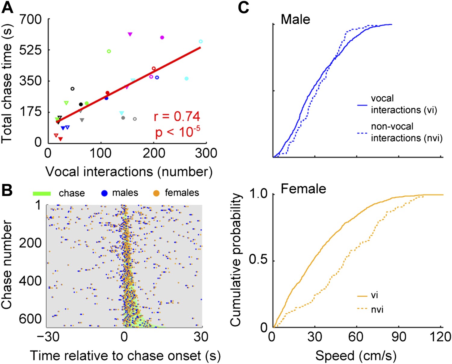
Vocal interactions are associated with courtship.
(A) The number of male-vocalization-initiated vocal interactions and total chase time for a given male-female pair was strongly correlated (n = 28; r = 0.74, p < 10−5). Trend line (red line) was calculated using linear regression. Circles and triangles represent male 1 and male 2, respectively. Open and filled depict female 1 and female 2, respectively. Colors indicate group numbers (black = 1, blue = 2, green = 3, red = 4, gray = 5, pink = 6, and cyan = 7). (B) Plots of male and female USVs as a function of time relative to chase. Vocal interaction rate is higher during chases than outside chases for male-initiated vocal interactions (p < 10−21). (C) Mouse speeds at the time of the male vocalization during chases with and without vocal interactions. Top, male speed (p > 0.25). Bottom, female speed (p < 10−10).
Figure 8
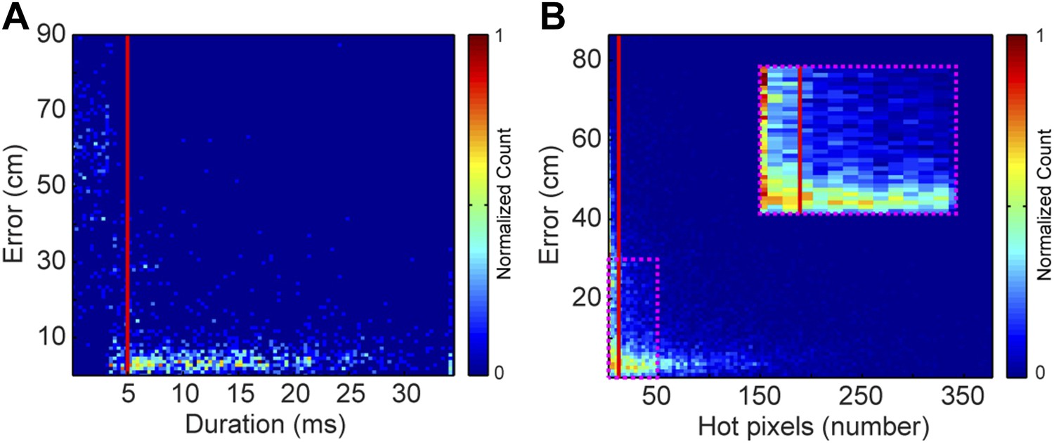
Effects of acoustic structure on localization fidelity.
(A) Localization error as a function of sound duration. The heat map shows that signals shorter than 5 ms (red vertical line) produce large errors between the estimated sound source location and the true position of the mouse. (B) Localization error as a function of hot pixel count (pixels in the sound's spectrogram that are significantly above background). Localization error is variable when the hot pixel count is low, and becomes more accurate above 11 hot pixels (red vertical line). Inset (dashed magenta box) shows zoomed in region of heat map highlighting the increase in localization error for snippets with fewer than 11 hot pixels. Heat maps were normalized by peak counts.
Tables
Table 1
Vocal Signals detected, localized, and assigned for each data set
| Session | Signals | Localized | Assigned | Individual male 1 | Male 2 | Female 1 | Female 2 | Proportion assigned* |
|---|---|---|---|---|---|---|---|---|
| 1 | 23,292 | 17,444 | 2115 | 1021 | 465 | 364 | 265 | 0.12 |
| 2 | 25,942 | 19,531 | 3118 | 1903 | 505 | 356 | 354 | 0.16 |
| 3 | 26,395 | 19,889 | 3690 | 2345 | 769 | 359 | 217 | 0.19 |
| 4 | 31,371 | 25,147 | 4201 | 2957 | 415 | 497 | 332 | 0.17 |
| 5 | 35,274 | 28,075 | 6337 | 4428 | 1054 | 471 | 384 | 0.23 |
| 6 | 52,597 | 40,483 | 6416 | 2747 | 2279 | 650 | 740 | 0.16 |
| 7 | 60,525 | 48,719 | 11,484 | 5608 | 4038 | 1084 | 754 | 0.24 |
-
*
Proportion assigned is based on number of localized signal.
Download links
A two-part list of links to download the article, or parts of the article, in various formats.
Downloads (link to download the article as PDF)
Open citations (links to open the citations from this article in various online reference manager services)
Cite this article (links to download the citations from this article in formats compatible with various reference manager tools)
Female mice ultrasonically interact with males during courtship displays
eLife 4:e06203.
https://doi.org/10.7554/eLife.06203


