Functional topography of the human entorhinal cortex
- Radboud University, Netherlands
- Radboud University Medical Centre, Netherlands
- University of Oxford, United Kingdom
Figures
Figure 1 with 1 supplement
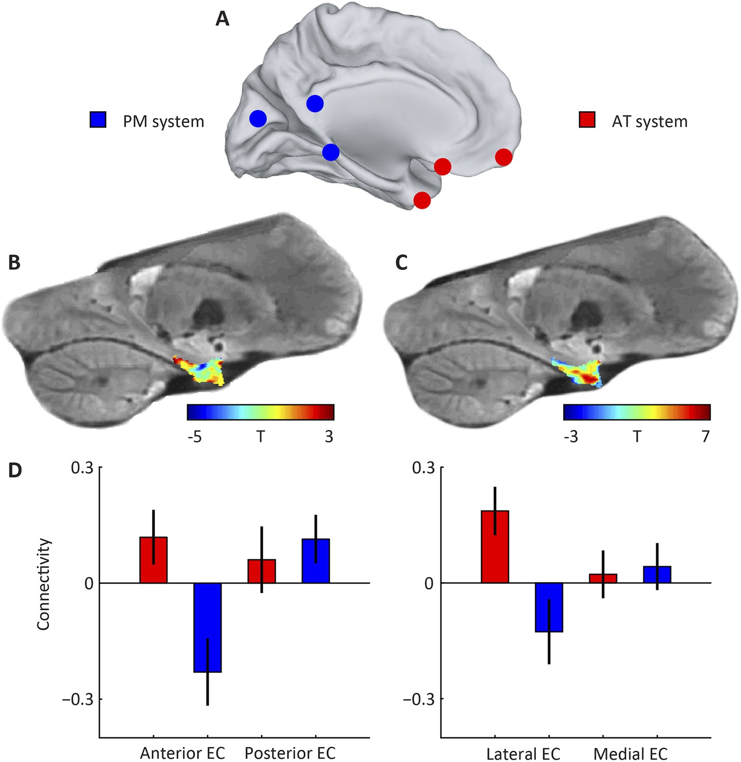
Subdivisions of entorhinal cortex (EC) and connectivity to anterior-temporal (AT) and posterior-medial (PM) cortical networks.
(A) Schematic of the AT and PM system. Spherical regions-of-interest (ROIs) were centred on MNI coordinates associated with either of the two systems (Libby et al., 2012), normalised to the group-specific template of the navigation study and then masked to include only gray matter voxels. The AT system included medial-prefrontal and orbitofrontal regions, whereas the PM system included occipital and posterior-parietal regions, see Table 1 for all selected regions. (B) Right parasagittal slice showing voxel-wise seed-based connectivity of the PM system restricted to the EC. Note the PM peak. (C) Right parasagittal slice showing voxel-wise seed-based connectivity of the AT system restricted to the EC. Note a peak in the anterior-lateral EC. (D) ROI-based connectivity estimates. Left panel: Connectivity strength (partial correlation coefficient) of anterior (left) and posterior EC (right) is plotted separately for the AT system (red) and the PM system (blue). The systems differ in their entorhinal connectivity: the anterior EC connects stronger to the AT compared to the PM network. Right panel: Connectivity strength with lateral (left) and posterior EC (right) is plotted separately for the AT system (red) and the PM system (blue). Lateral EC connected stronger to the AT compared to the PM network. Error bars show S.E.M. over subjects. See Figure 1—figure supplement 1 for additional slices.
Figure 1—figure supplement 1
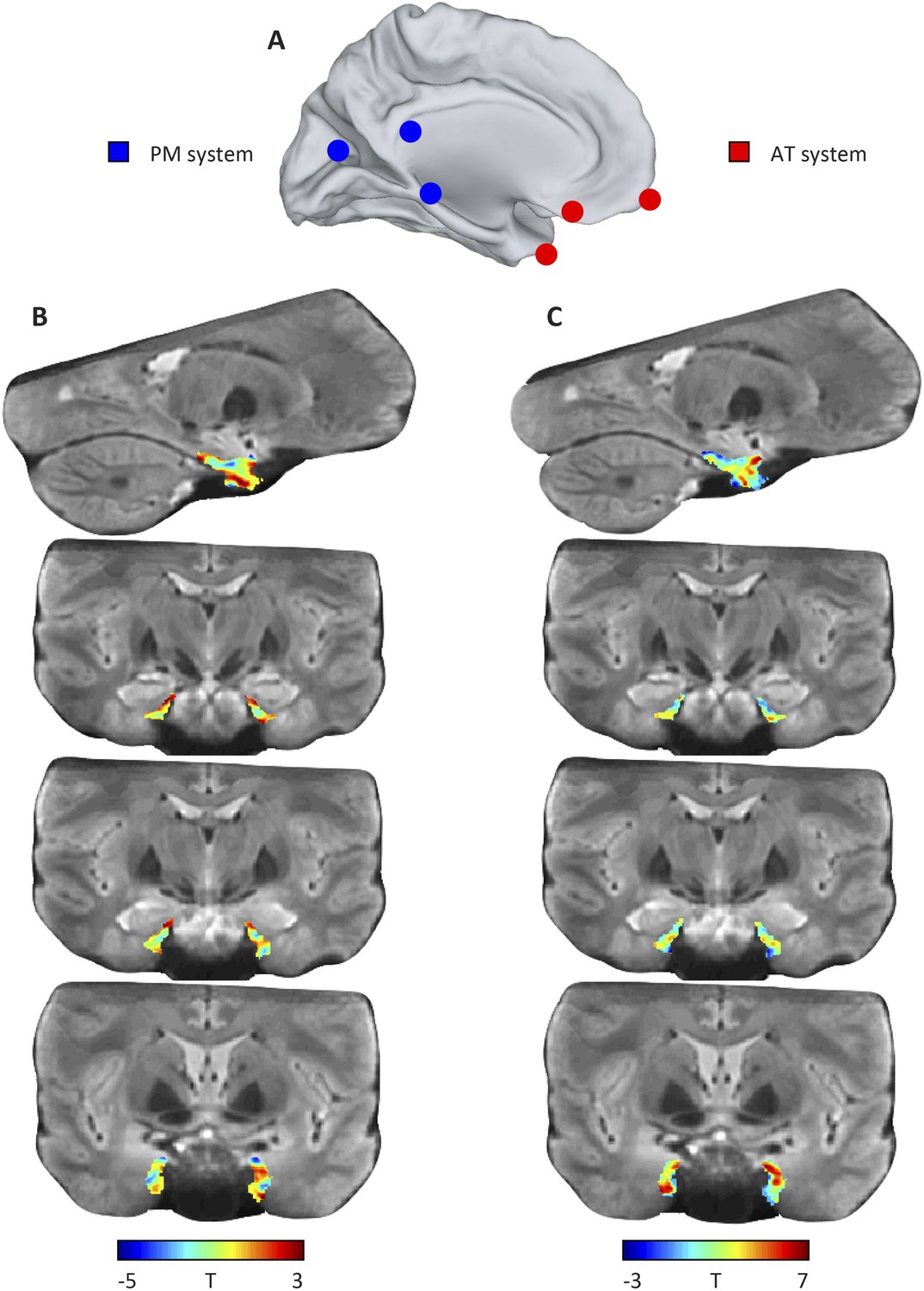
Results of the model-based connectivity analyses (additional slices).
(A) Schematic of the AT and PM system. (B) Top row: left parasagittal slice showing connectivity with the PM network. Bottom rows: coronal slices showing connectivity with the PM network. (C) Top row: left parasagittal slice showing connectivity with the PM network. Bottom rows: coronal slices showing connectivity with the PM network.
Figure 2 with 4 supplements
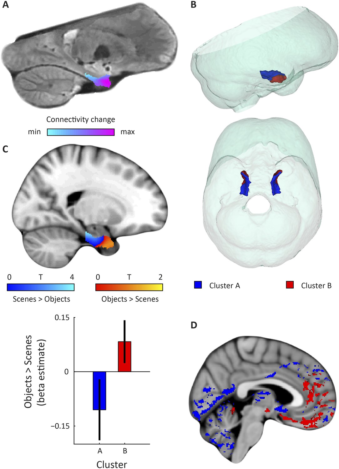
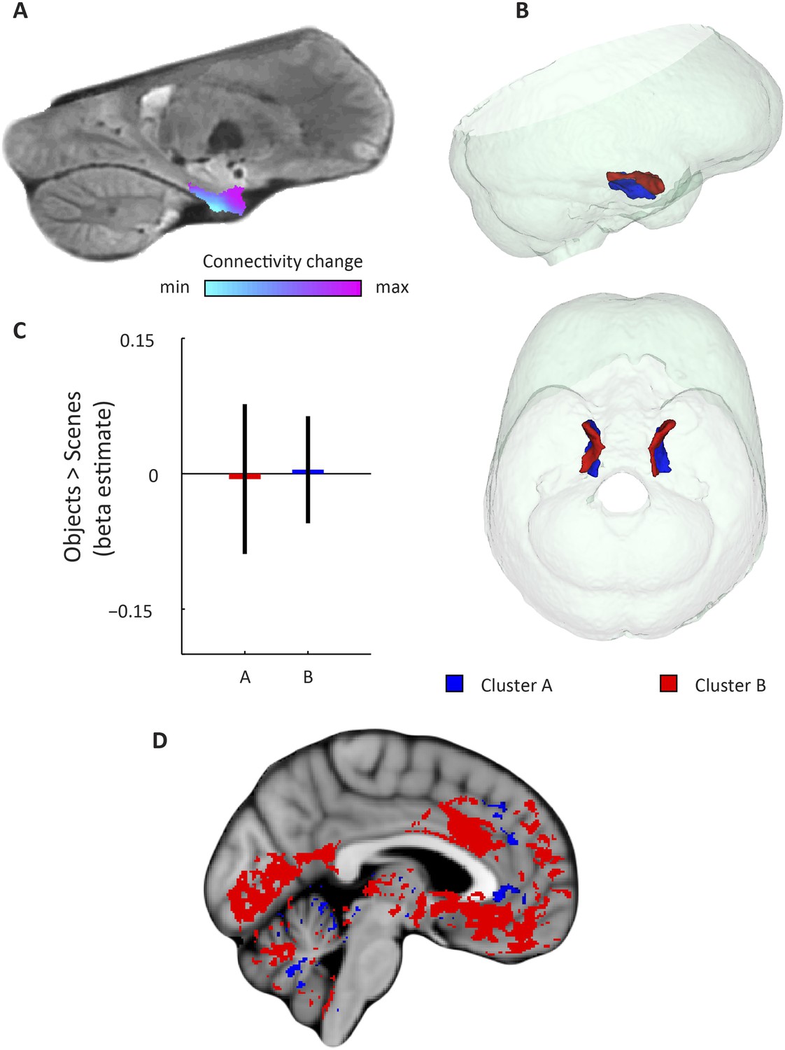
Dominant mode of functional connectivity change within EC and sensitivity to spatial and non-spatial information.
(A) Dominant mode of functional connectivity change at the group-level (Spearman's R = 0.53). Similar colours indicate similar connectivity with the rest of the brain. (B) 3D rendering of the two clusters derived from the dominant mode of functional connectivity change (displayed in red and blue) and the outlines of the group-specific template. Upper panel: right side view. Lower panel: top view (see Figure 2—figure supplement 1 for coronal views of the two clusters). (C) Upper panel: Map shows results of a non-parametric randomisation test of the spatial and non-spatial stimulation experiment restricted to the EC for display purposes (see Figure 2—figure supplement 2 for whole-brain maps). The ‘scenes > objects’ contrast is displayed in blue to light-blue, the ‘scenes < objects’ contrast in red to yellow. Note that voxels in pmEC are sensitive to scenes, whereas voxels in alEC are sensitive to objects. Lower panel: The clusters from panel B exhibit antagonistic responses to spatial and non-spatial stimuli. Beta estimates for the contrast ‘scenes > objects’ (averaged across participants) are shown for clusters A and B. T(20) = 4.9, p = 0.0001. Error bars show S.E.M. over participants. (D) Whole-volume functional connectivity with clusters A and B. Regions connecting more with cluster A (p < 0.05, FWE corrected), such as occipital and posterior-parietal cortex that form part of the PM system are shown in blue. Regions connecting more with cluster B (p < 0.05, FWE corrected), such as medial-prefrontal and orbitofrontal cortex which form part of the AT system are displayed in red.
Figure 2—figure supplement 1
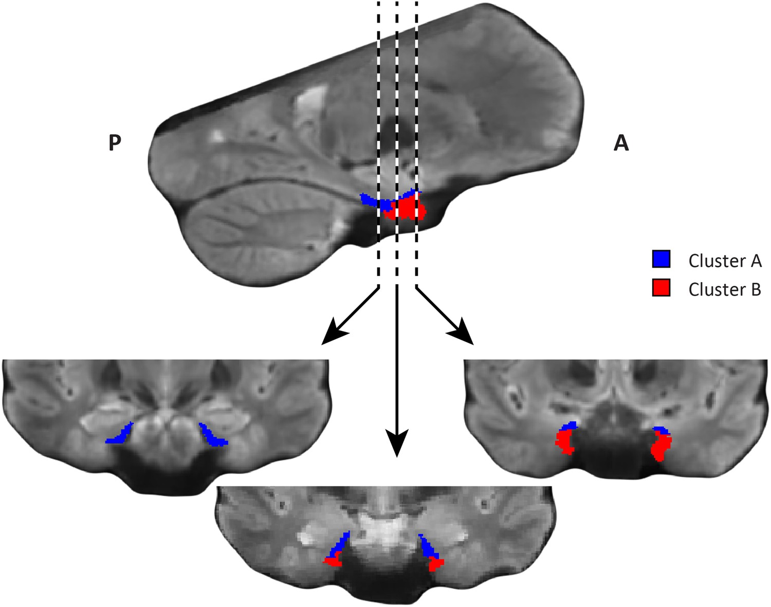
Coronal views of the two clusters.
Top: sagittal slice. Dashed lines indicate position of the coronal slices shown below. Bottom: The posterior slice (left) exclusively contains cluster A. In the middle slice cluster A is located dorsomedially, proximal to the hippocampus and cluster B is located ventrolaterally, distal to the hippocampus. The anterior slice (right) contains mostly cluster B. A = anterior; P = posterior.
Figure 2—figure supplement 2
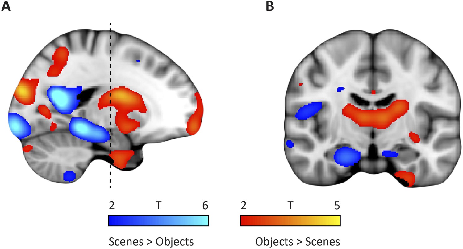
Whole-brain modulation by spatial and non-spatial stimuli.
(A) Left parasagittal slice showing peak effects of two contrasts on the data from the spatial and non-spatial stimulation experiment. The ‘scenes > objects’ contrast is displayed in blue-lightblue, the ‘scenes < objects’ contrast in red-yellow. Note that voxels in the posterior EC are sensitive to scenes, whereas voxels in the anterior EC are sensitive to objects. (B) Coronal slice anterior-posterior location indicated by dashed line in (A). Note the medial peak in the medial temporal lobe for the ‘scenes > objects’ contrast and the lateral peak for the ‘scenes < objects’ contrast. Images are thresholded at T > 2 for display purposes.
Figure 2—figure supplement 3
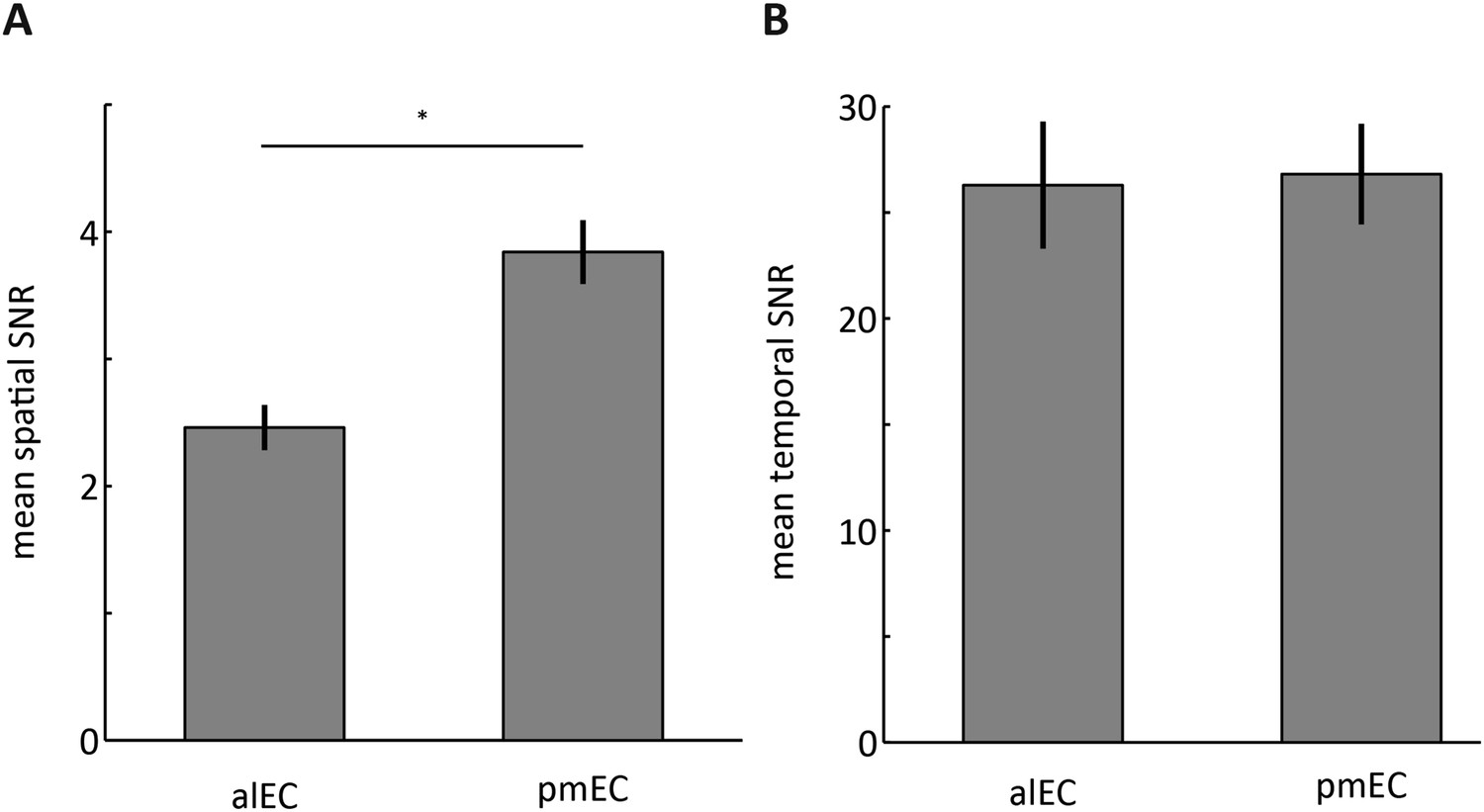
Signal-to-noise ratios (SNRs) in the alEC and pmEC.
(A) Bar plots of the ratio between the mean signal intensity and signal standard deviation across voxels. The SNR across voxels was higher in the pmEC than the alEC (T(21) = 15.2721, p < 0.001). This was associated with a larger signal in the pmEC (mean signal alEC = 4.97; mean signal pmEC = 7.76; T(21) = 38, p < 0.001) in the absence of differences in spatial standard deviation (T(21) = 1.5, p = 0.144). Note, that mean signal was subtracted from time-series prior to all connectivity analyses (see ‘Materials and methods’), which makes it unlikely that signal intensity differences affected the connectivity results. (B) Bar plots of the ratio between the mean signal intensity and the signal standard deviation across time. Temporal SNR (tSNR) did not differ between alEC and pmEC (T(21) = 0.2, p = 0.83). Error bars show S.E.M. over participants.
Figure 2—figure supplement 4

Homologous and non-homologous connectivity of the alEC and the pmEC.
Connectivity between subregions identified using the data-driven connectivity analysis. Connectivity reflects partial Pearson correlation coefficients after Fisher Z transformation. Laterality is indicated by the last letter: left = ‘l’, right = ‘r’. (B) Connectivity for three conditions. ‘non-hom’ refers to non-homologous connectivity, ‘contra’ refers to contralateral connectivity and ‘hom’ refers to homologous connectivity. Note that homologous connectivity (across hemispheres) exceeded connectivity with the neighbouring non-homologous region in the same hemisphere (T(21) = 4.05, p = 0.0006). Connectivity between non-homologous regions was strongest within hemispheres (T(21) = 3.66, p = 0.0015). Error bars show S.E.M. over participants. *p < 0.05.
Figure 3 with 1 supplement
Second-dominant mode of functional connectivity change within EC and sensitivity to spatial and non-spatial information.
(A) Second-dominant mode of functional connectivity change at the group-level (Spearman's R = 0.28). Similar colours indicate similar connectivity with the rest of the brain. (B) 3D rendering of the two clusters derived from the second-dominant mode of functional connectivity change (displayed in red and blue) and the outlines of the group-specific template. Upper panel: right side view. Lower panel: top view (see Figure 3—figure supplement 1 for coronal views of the two clusters). (C) The clusters shown in panel B exhibit no antagonistic responses to spatial and non-spatial stimuli. Beta estimates for the contrast ‘scenes > objects’ (averaged across participants) are shown for cluster A and B (T(20) = −0.26, p = 0.8). Error bars show S.E.M. over participants. (D) Regions connecting more with cluster A (p < 0.05, FWE corrected) are shown in blue. Regions connecting more with cluster B (p < 0.05, FWE corrected) are shown in red. Cluster A connected more with most of the neocortex.
Figure 3—figure supplement 1

Coronal views of the two clusters.
Top: sagittal slice. Dashed lines indicate position of the coronal slices shown below. Bottom: All three coronal slices contain both clusters. Cluster A is located ventrally, distal to the hippocampus and cluster B dorsally, proximal to the hippocampus. A = anterior; P = posterior.
Figure 4
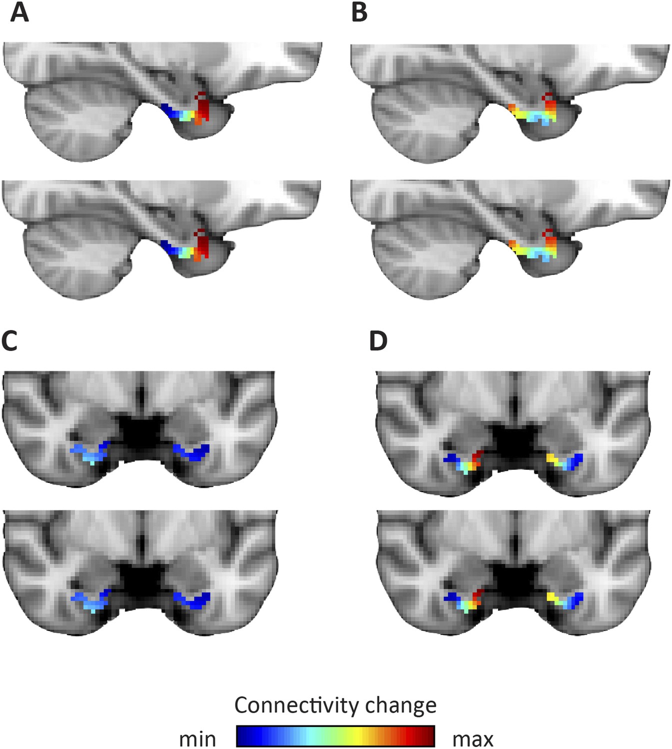
Dominant and second-dominant modes of functional connectivity change on the basis of resting-state functional magnetic resonance imaging.
Results of analysis of the first 60 participants of the WU-Minn Human Connectome Project (HCP), acquired on two different days (Smith et al., 2013). Top row: day one. Bottom row: day two. (A, C) The dominant mode of functional connectivity change follows an anteroposterior trajectory. (B, D). The second-dominant mode of functional connectivity change follows a mediolateral trajectory. Both modes were highly reproducible across different scanning days (dominant mode: Pearson's R = 0.99 p < 0.001, second-dominant mode: R = 0.98; p < 0.001). Topology preservation—dominant mode, day one: Spearman's R = 0.62; day two: R = 0.61; second-dominant mode, day one: R = 0.44; day two: R = 0.46.
Figure 5
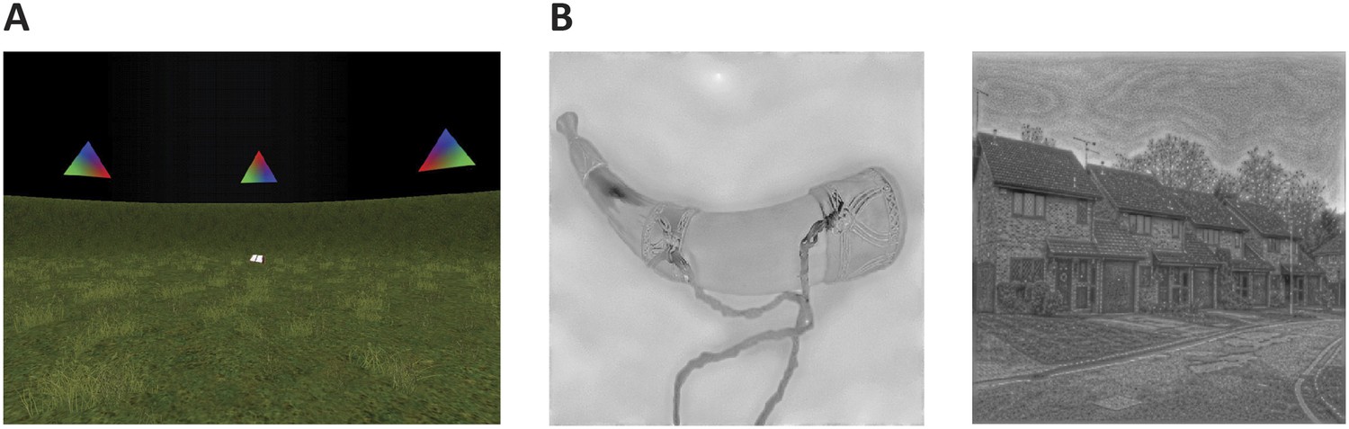
Cognitive tasks.
(A) Navigation experiment. First person view of the virtual arena that participants navigated freely to perform the object-location memory task. (B) Spatial and non-spatial stimulation. Left: An example stimulus of a ‘non-spatial’ object. Right: An example stimulus of a ‘spatial’ scene.
Author response image 1
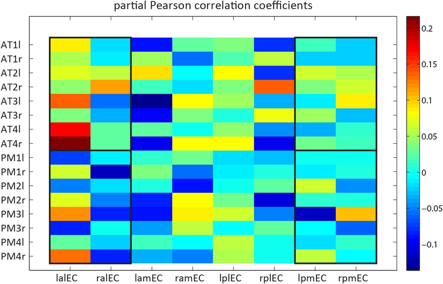
Detailed model-based connectivity analyses. Single spheres to EC quadrants across hemispheres.
Functional connectivity (partial correlation coefficients) of spherical ROIs of 4 mm radius, centred on a bilateral selection of coordinates reported by Libby et al. (2012) to 4 EC subregions in both hemispheres. The non-overlapping EC subregions were segmented manually. X-axis labels: the first letter indicates laterality (l vs r), the second anterioposterior location (a vs p), the third mediolateral location (m vs l). Y-axis labels: AT1 = Anterior inferior temporal gyrus; AT2 = Perirhinal cortex; AT3 = Dorsolateral prefrontal cortex; AT4 = Orbitofrontal cortex; PM1 = Medial posterior occipital cortex; PM2 = Retrosplenial cortex; PM3 = Occipital pole; PM4 = parahippocampal cortex. Last letter indicates laterality (l vs r).
Videos
Video 1
3D rendering of the two clusters derived using the dominant mode of functional connectivity change. Cluster A is shown in red and cluster B in blue.
https://doi.org/10.7554/eLife.06738.014Tables
Table 1
Selection of regions associated with the posterior-medial (PM) and the anterior-temporal (AT) system (Libby et al., 2012).
The coordinates of the PM system reflect peak voxel coordinates of a seed-based connectivity contrast of right parahippocampal cortex > right perirhinal cortex connectivity reported by Libby et al. (Libby et al., 2012). The coordinates of the AT system reflect peak voxel coordinates of a seed-based connectivity contrast of right perirhinal cortex > right parahippocampal cortex connectivity. Coordinates are in MNI space.
| Left hemisphere | Left hemisphere | |||||
|---|---|---|---|---|---|---|
| x | y | z | x | y | z | |
| PM System | ||||||
| Medial posterior occipital cortex (BA 18) | – | – | – | 14 | −72 | 8 |
| Occipital pole (BA 17) | −16 | −96 | 22 | – | – | – |
| Parahippocampal cortex | −12 | −42 | −8 | 22 | −32 | −8 |
| Posterior cingulate cortex (BA 29) | −4 | −46 | 4 | 10 | −44 | 10 |
| Posterior hippocampus | −20 | −30 | −2 | 18 | −36 | 0 |
| Posterior thalamus | −20 | −34 | 0 | 22 | −30 | 6 |
| Retrosplenial cortex (BA 30) | −16 | −52 | −4 | 22 | −46 | 0 |
| AT System | ||||||
| Dorsolateral prefrontal cortex (BA 9) | −24 | 60 | 24 | 18 | 58 | 24 |
| Dorsomedial prefrontal cortex (BA 8) | −2 | −60 | 34 | – | – | – |
| Frontal polar cortex (BA 10) | – | – | – | 40 | 60 | −2 |
| Lateral precentral gyrus (BA 6) | – | – | – | 54 | 4 | 10 |
| Medial prefrontal cortex (BA 8) | −2 | −60 | 34 | – | – | – |
| Orbitofrontal cortex (BA 11/47) | −6 | 16 | −22 | 8 | 22 | −20 |
| Postcentral gyrus (BA 4) | – | – | – | 62 | −10 | 16 |
| Posterior superior temporal gyrus (BA 22) | −62 | −34 | 14 | – | – | – |
| Rostrolateral prefrontal cortex (BA 10) | – | – | – | 38 | 60 | −12 |
| Temporal polar cortex (BA 38) | – | – | – | 34 | 22 | −36 |
| Ventrolateral prefrontal cortex (BA 44/45) | −56 | 6 | 18 | – | – | – |
Download links
A two-part list of links to download the article, or parts of the article, in various formats.
Downloads (link to download the article as PDF)
Open citations (links to open the citations from this article in various online reference manager services)
Cite this article (links to download the citations from this article in formats compatible with various reference manager tools)
Functional topography of the human entorhinal cortex
eLife 4:e06738.
https://doi.org/10.7554/eLife.06738


