Irregular spiking of pyramidal neurons organizes as scale-invariant neuronal avalanches in the awake state
- National Institute of Mental Health, United States
Figures
Figure 1 with 2 supplements
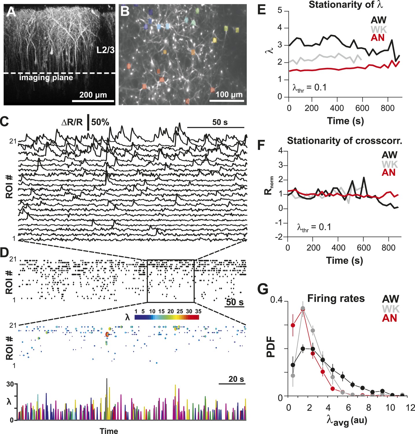
Imaging of ongoing spiking activity in groups of L2/3 PNs in the awake (AW) rat.
(A) Z-stack side projection of YC2.60-expressing PNs in L2/3 in vivo. (B) Single imaging plane (dotted line in A) containing a group of PNs with significant changes in fluorescent intensity ∆R/R over time (colored ROIs). (C) Time course of ΔR/R for individual ROIs (from B). (D) Top: Binary raster display of instantaneous spike rate estimate λ (λthr = 0.1). Middle: Expanded period showing color coded λ amplitude. Bottom: Overplot of λ time course for individual, color-coded ROIs. (E, F) Stationary firing rate estimate λ and pairwise crosscorrelation Rnorm (normalized by the correlation during the first 30 s) over the course of acquisition. Firing rate increased from anesthetized to AW conditions but remained stable throughout the recording, suggesting that our measures were not affected by slow modulations of activity (Ecker et al., 2010). Shown are averages over all PN groups. (G) Distributions of the average firing rate estimate, λavg, for the three different states.
Figure 1—figure supplement 1
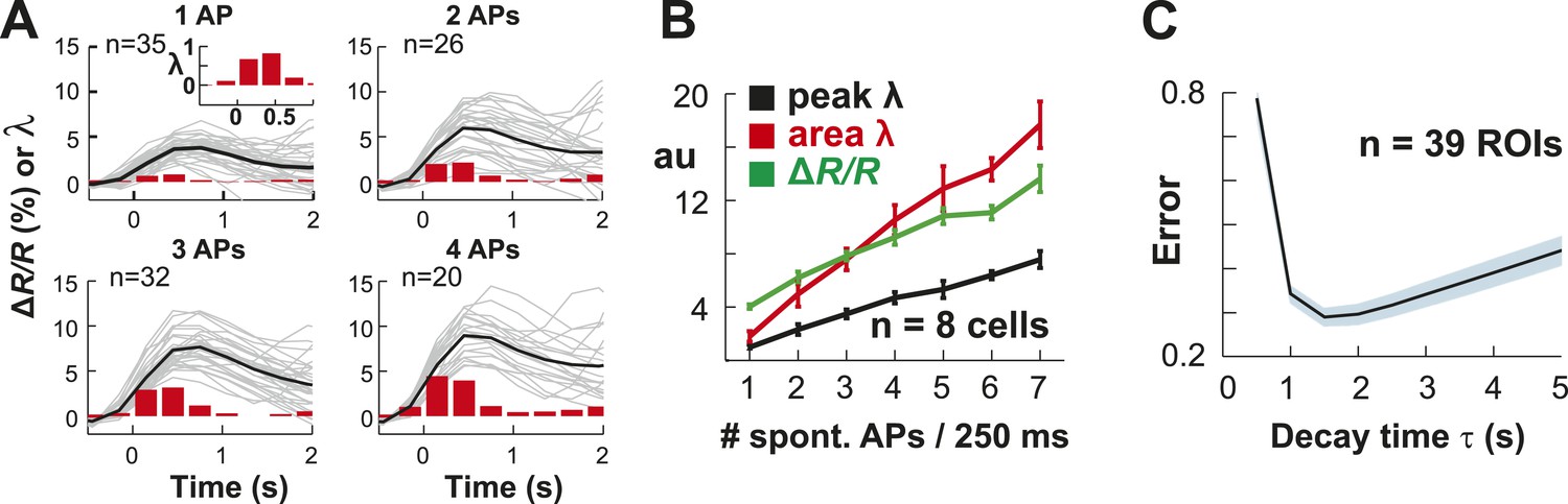
Single AP detection in YC2.60-expressing neurons at physiological temperature and performance of the OOPSI deconvolution algorithm.
(A) Using whole-cell patch recording of YC2.60-expressing PNs in cortical slice cultures, we confirmed that YC2.60 reliably resolved spontaneous single AP firing at physiological temperature (∼32°C), in line with previous reports (Yamada et al., 2011). Gray: Individual trials: Black: Average. Inset: Zoomed view of bar graph from 1 AP subpanel. Note the decay in ΔR/R by ∼2/3 within 1–2 s. Responses from single PN. (B) Peak and integral of instantaneous rate λ as well as peak ΔR/R linearly increase with the number of spontaneous APs/250 ms (n = 7 neurons). (C) Single movie data showing that the minimum reconstruction error of the deconvolution was found at decay time τ = 1.5 s (n = 39 ROIs).
Figure 1—figure supplement 2
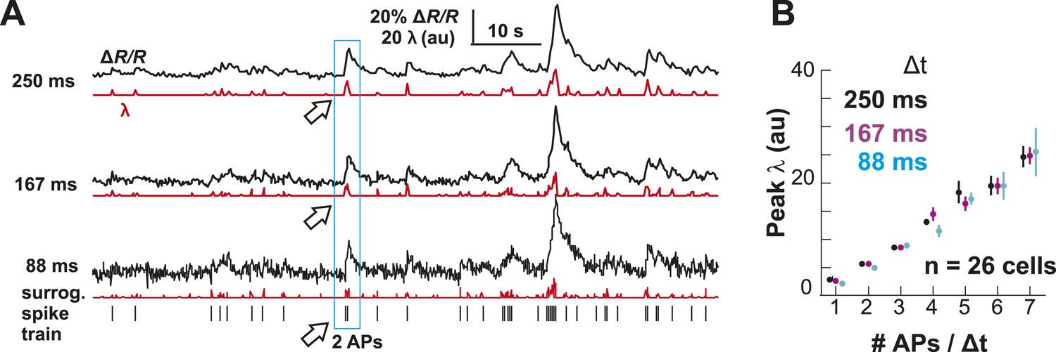
Performance of the OOPSI deconvolution algorithm at different temporal resolutions and noise levels.
(A) Surrogate intracellular calcium traces (ΔR/R; black) and corresponding λ estimates (red) at three temporal resolutions Δt. ΔR/R was derived by convolution of an in vivo spike train (bottom) with the instantaneous calcium response (τ = 1.5 s; 5% peak amplitude for one AP; for details see ‘Materials and methods’). (B) Peak λ linearly increases with the number of APs/Δt.
Figure 2 with 1 supplement
Spatial and temporal clustering in ongoing spiking activity in vivo.
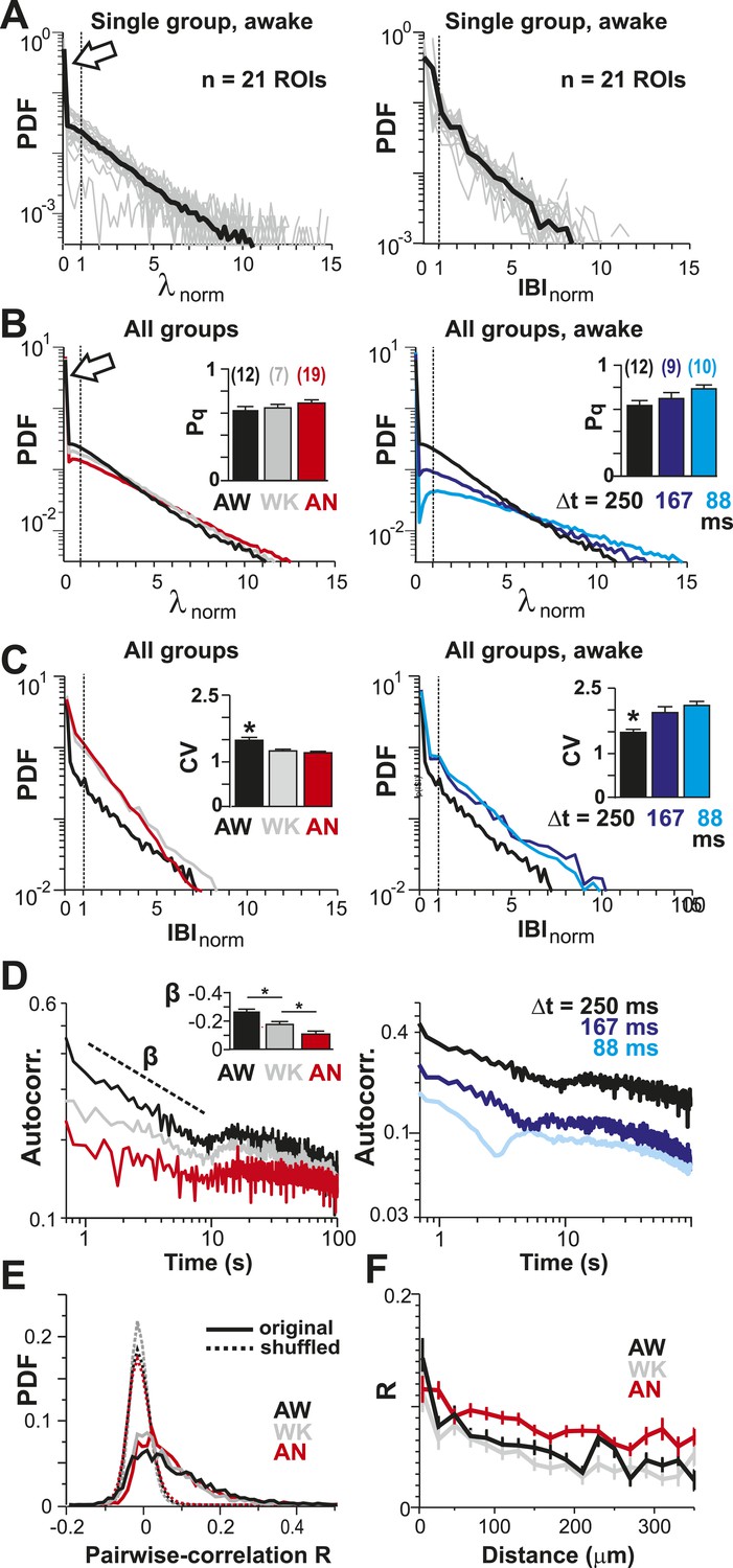
(A) Probability distributions of λnorm = λ/λavg (left) and distribution of normalized quiescent time intervals, IBInorm = IBI/IBIavg, (right) in the AW state for a single neuronal group of PNs (Δt = 250 ms). Gray: distributions for individual ROIs, black: average. Dotted lines, λnorm = 1 and IBInorm = 1. The arrow is pointing at the relatively high-probability function value for λnorm << 1, that is, no spike within Δt = 250 ms. Note that the transition from ‘no spike’ to spiking is rather abrupt in the distribution, which indicates the high signal-to-noise ratio in our recorded data (cf. Figure 1—figure supplement 1A,B). (B) Average λnorm distributions over all PN groups for all three conditions (left; AW; WK, waking; AN, anesthetized) and temporal resolutions (right). Inset: probability of quiescence Pq (number of recordings is indicated in parentheses). (C) Distribution of IBInorm for all three conditions (left) and temporal resolutions (right). Inset: Coefficient of variation (CV) for IBI (*p < 0.05). (D) Average autocorrelation function for λ across PNs for all three conditions (left; Δt = 250 ms) and temporal resolutions (right). Inset: Power-law exponent β (*p < 0.05). Note steeper power-law decay for AW indicating increased temporal clustering. (E) Distribution of pairwise crosscorrelation, R, in λ for all PN groups and different states. Broken lines: Corresponding independent model by shuffling λ for each ROI. (F) AW shows steeper distance decay in R when compared to AN indicating higher spatial clustering.
Figure 2—figure supplement 1
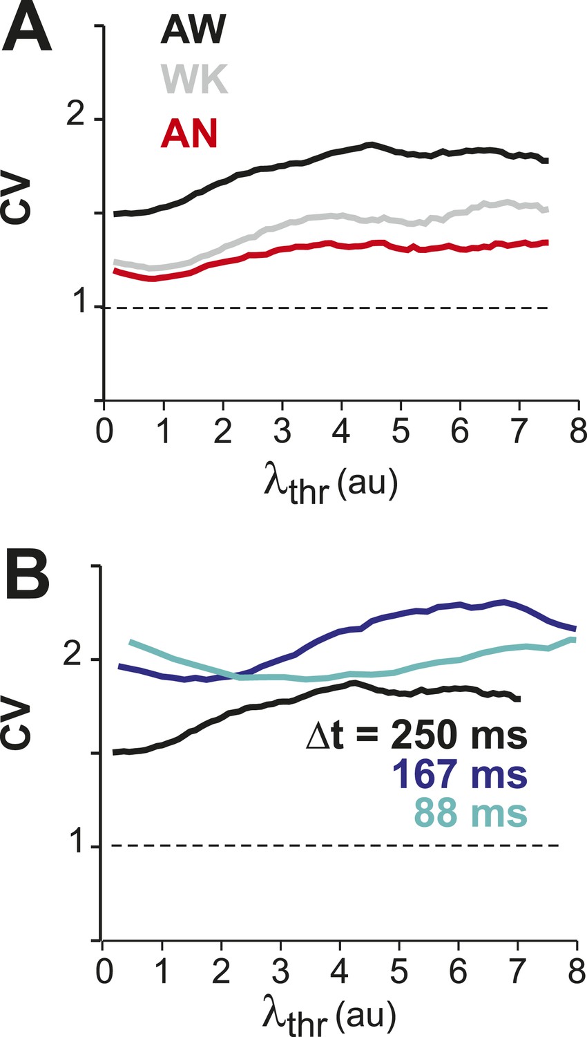
CV in λ remains larger than one for increasing λthr for all conditions (A) and temporal resolutions (B).
https://doi.org/10.7554/eLife.07224.007
Figure 3
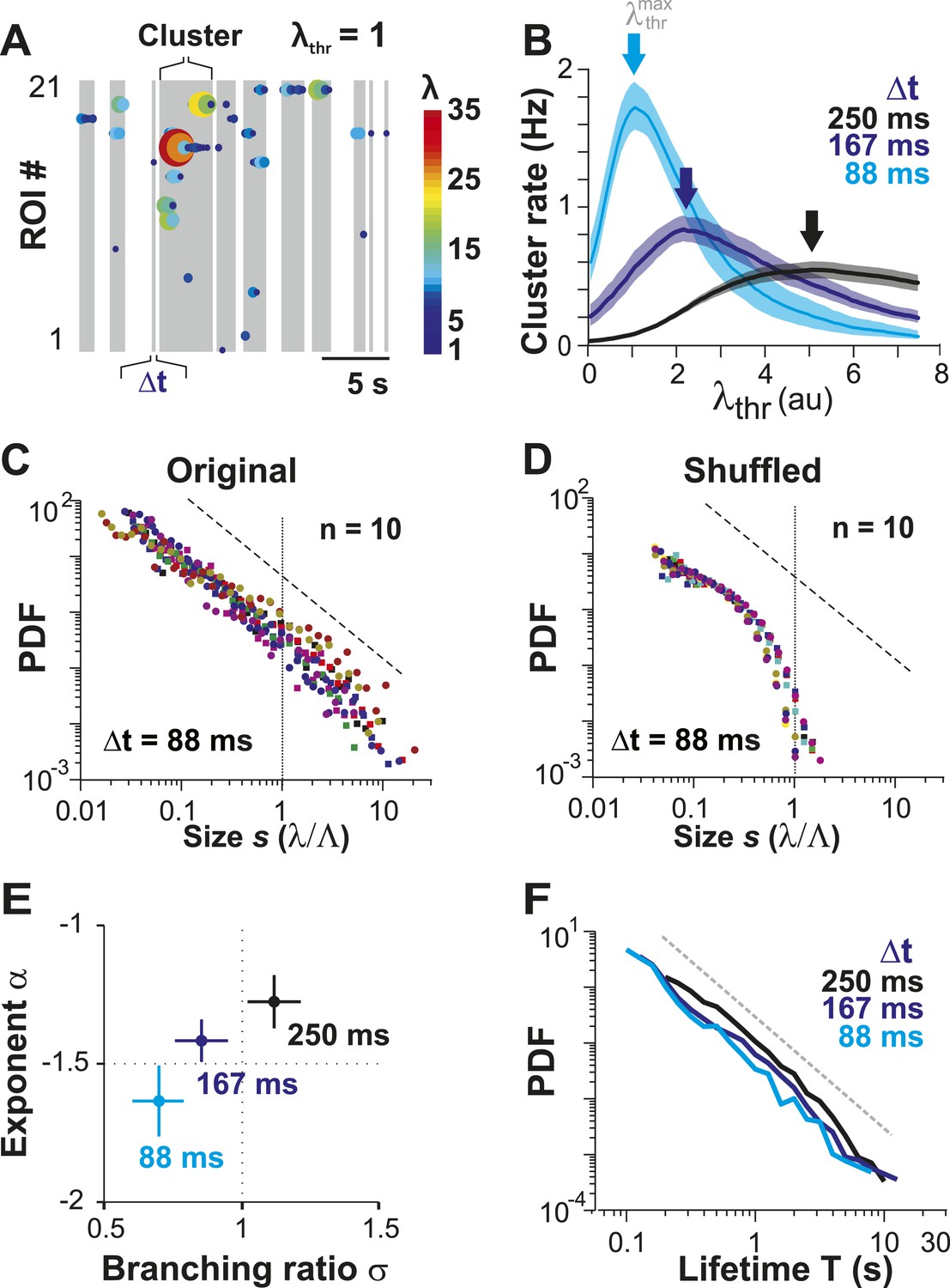
Ongoing spiking in local PNs organizes as neuronal avalanches in vivo.
(A) Sketch of cluster formation at given Δt and chosen λthr = 1. Gray boxes delineate clusters of activity (i.e., consecutive time bins with λ > λthr). (B) Maximal cluster rate at intermediate λthr for different Δt in the AW condition. Vertical arrows indicate the respective at which cluster rate is maximal. (C) Individual distributions of normalized cluster sizes, s, in AW (top; Δt = 88 ms, n = 10 recordings, threshold at ). Dotted line, predicted cut-off at s = 1; dashed line, power law with α = −1.5. (D) Corresponding distributions after shuffling λ. Shuffling destroys spatiotemporal correlations in activity and abolishes the power law in cluster sizes. (E) Relationship between α and branching ratio σ for all three temporal resolutions, Δt. Note the systematic change for increasing Δt as shown previously for avalanche dynamics based on the LFP. (F) Distribution of cluster lifetimes, T, for different Δt. Dashed line, slope = −2.
Figure 4
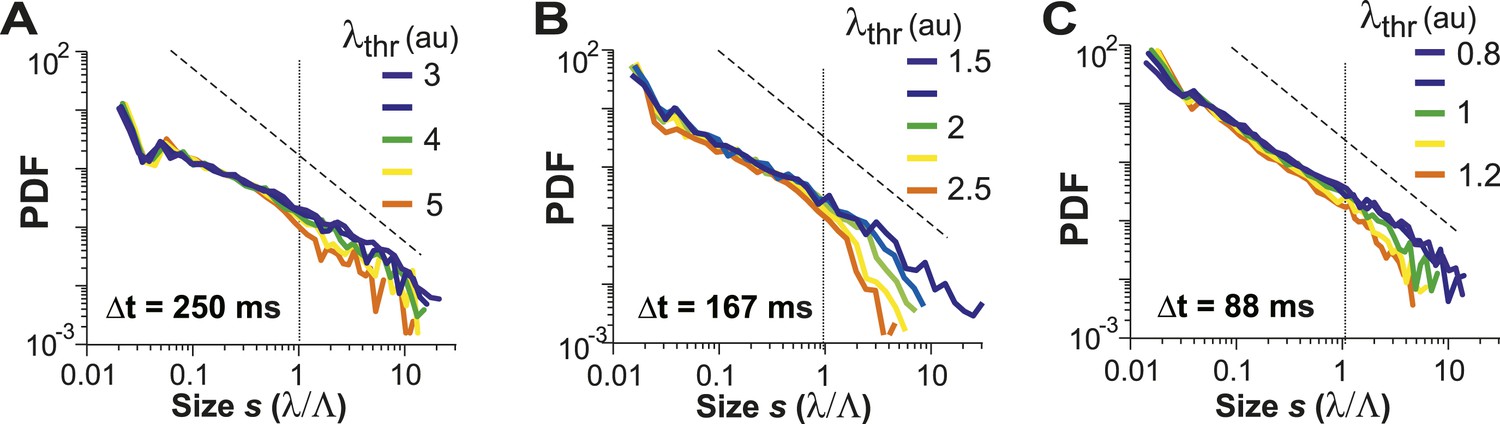
Avalanche dynamics is robust to changes in λthr.
(A–C) Cluster size distributions for Δt = 250, 167, and 88 ms (from left to right). The green distributions correspond to the respective thresholds, λthr = , at which the cluster rate was maximal.
Figure 5 with 1 supplement
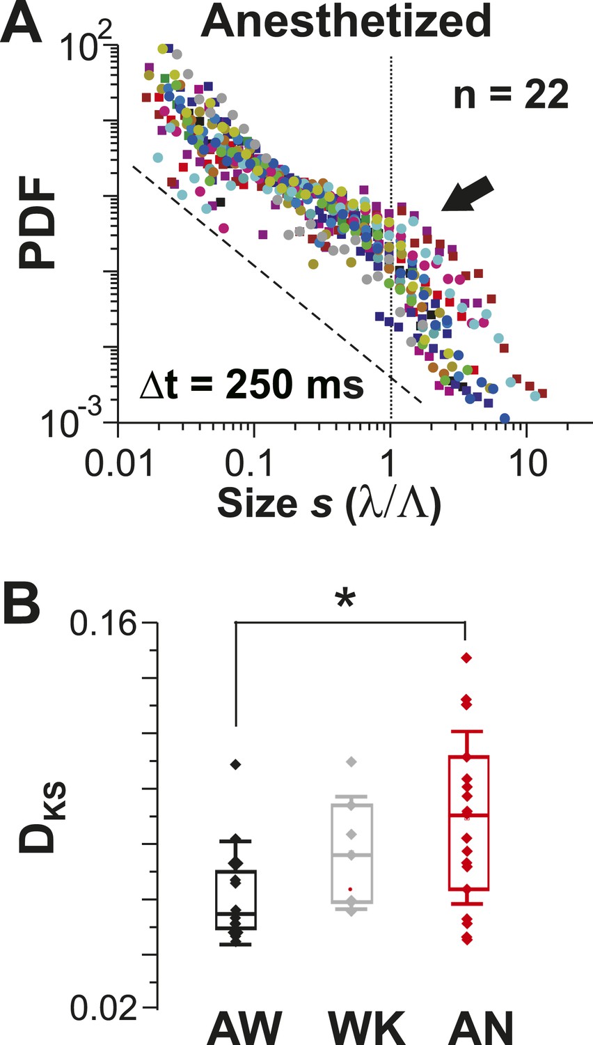
Avalanche dynamics is abolished under anesthesia.
(A) Overplot of size distributions for the anesthetized state (n = 22 recordings) showing a slight increase in the probability of large clusters (arrow). (B) Average KS distance, DKS, between individual PDFs and best-fit power-law distributions for all three states (*p < 0.05).
Figure 5—figure supplement 1
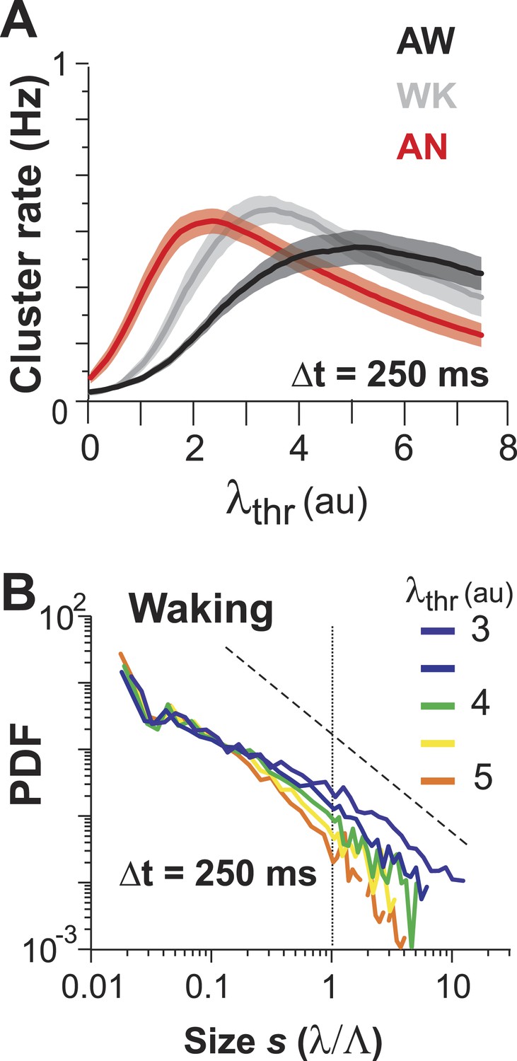
(A) Maximum cluster rate is observed at intermediate threshold levels for all three conditions.
(B) Average cluster size distributions as a function of λthr for WK.
Figure 6 with 1 supplement
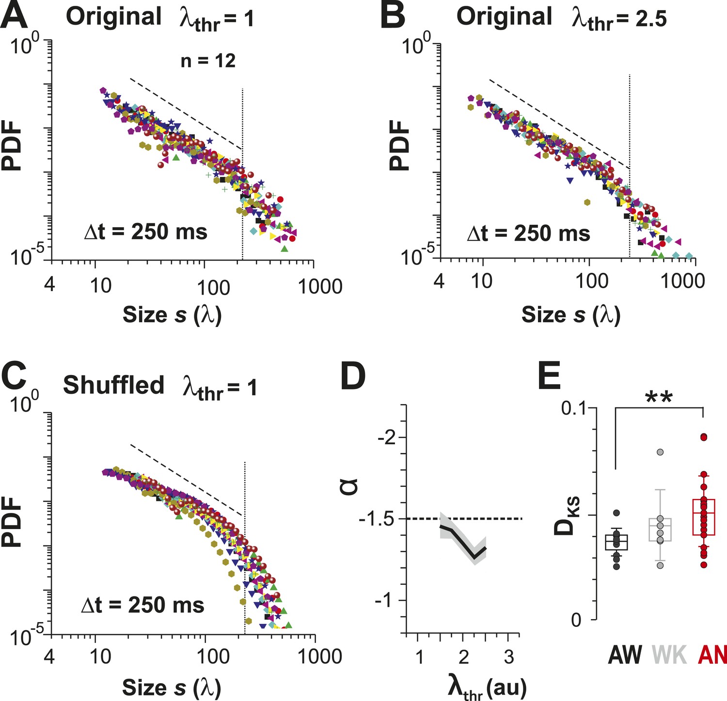
Identifying avalanche dynamics, that is, power law in clustering, using thresholding of the population rate vector (Poil et al., 2012).
(A, B) Cluster size distributions for individual recordings (n = 12) following thresholding of the population rate vector at λthr = 1 (A) and 2.5 (B). Dashed line: slope = −1.5. (C) Rate-preserved shuffling of λ in individual ROIs prior to calculation of population rate vector destroys the power law. (D) Power-law exponent, α, is relatively threshold-invariant. (E) Deviation from power-law dynamics at the population rate vector level increases with the transition from AW to AN (**p < 0.01).
Figure 6—figure supplement 1
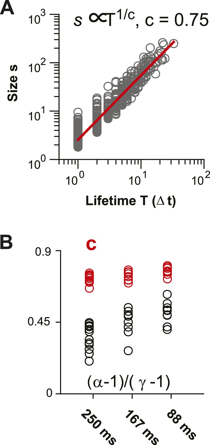
Scaling relationship between lifetime and size of spontaneous AP clusters supports neuronal avalanche dynamics (Sethna et al., 2001; Friedman et al., 2012).
(A) Double logarithmic plot of avalanche duration and corresponding avalanche size for one local L2/3 PN group in vivo in the AW state. Duration and size scale according to a power law with exponent 1/c. In this example, c was found to be 0.75 based on regression analysis (red line). (B) For increasing temporal resolution, the scaling relationship between life time exponent and size exponent approaches c.
Figure 7 with 3 supplements

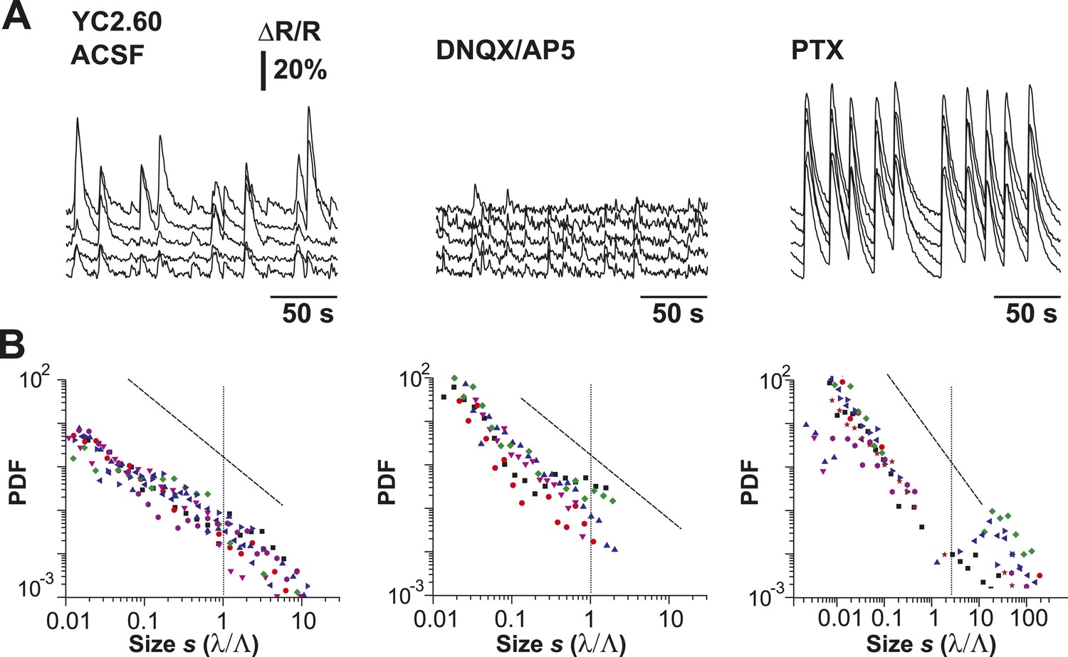
Spatiotemporal clustering in ongoing spiking activity recorded from groups of L2/3 PNs in vitro.
(A) Organotypic cortex (ctx)-ventral tegmental area (vta) co-culture. YC2.60-expression in PNs from superficial (super) but not deep (deep) cortical layers. wm: white matter border location. (B) Single imaging plane containing a group of PNs with significant changes in R over time (colored ROIs). (C) Time course of ΔR/R for individual ROIs. (D) Top: Binary raster display of instantaneous spike rate estimate λ (λthr = 0.1). Middle: Expanded period showing λ amplitudes. Bottom: Overplot of λ time course for individual (color coded) ROIs. (E) Distributions of λnorm for different pharmacological conditions (ACSF, DNQX/AP5, PTX). Dotted line, λnorm = 1. (F) Distributions of IBInorm. Dotted line, IBInorm = 1. Inset: Pq (number of recordings is indicated; *p < 0.05). (G) Mean λ autocorrelation function for individual PNs and different conditions. (H) Distance dependence of pairwise crosscorrelation in λ and different conditions. (I) Left: Power-law distributions in s for different λthr (color scale) for normal condition (ACSF). Right: λ shuffling destroys power-law organization for normal condition. (J) Probability distributions in s for different λthr (color scale) under PTX (left) and DNQX/AP5 (right). Dashed lines in I and J: slope = −1.5.
Figure 7—figure supplement 1
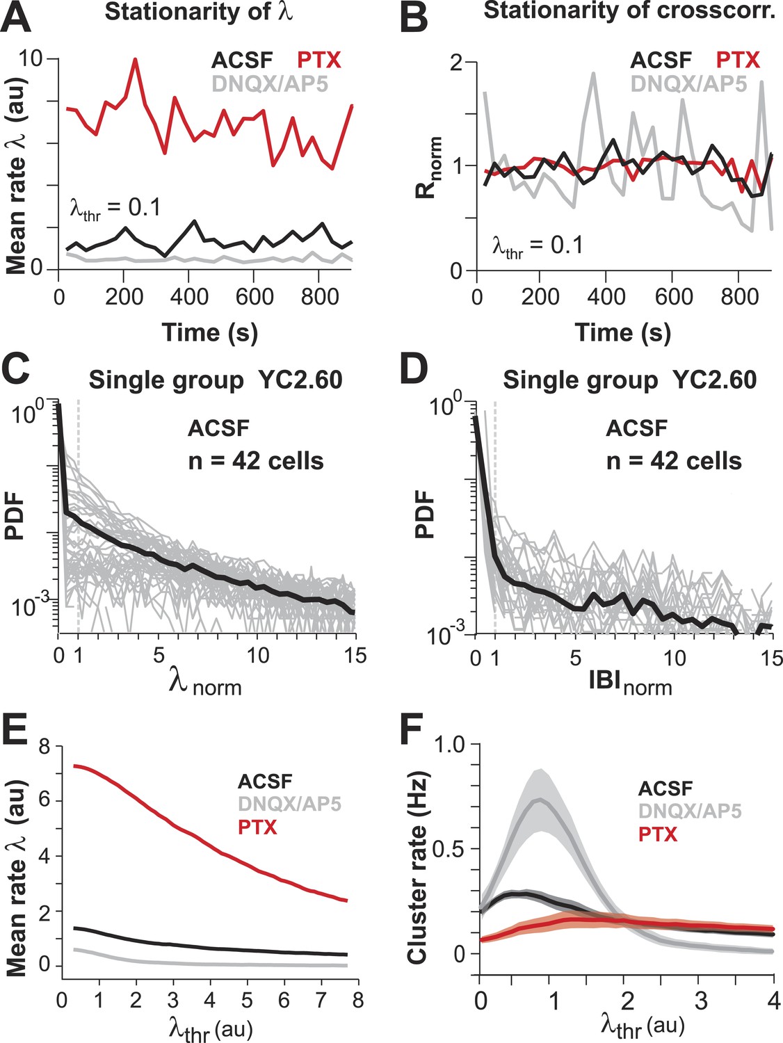
(A, B) Mean λ rate and pairwise crosscorrelation are stationary over entire imaging session.
(C, D) Distribution of normalized λ and IBIs for a single PN group (n = 42 ROIs). (E) Mean λ rate smoothly decreases with increasing threshold. (F) Cluster rate as function of λthr shows peak at intermediate λthr.
Figure 7—figure supplement 2
Cluster size distributions under normal condition, disfacilitation (DNQX/AP5), and disinhibition (PTX) for YC2.60.
(A) Example of simultaneously recorded fluorescent intensity ∆R/R over time for a subset of ROIs for all conditions using YC2.60 expressed in superficial cortical PNs. (B) Distributions of normalized cluster sizes for all conditions.
Figure 7—figure supplement 3
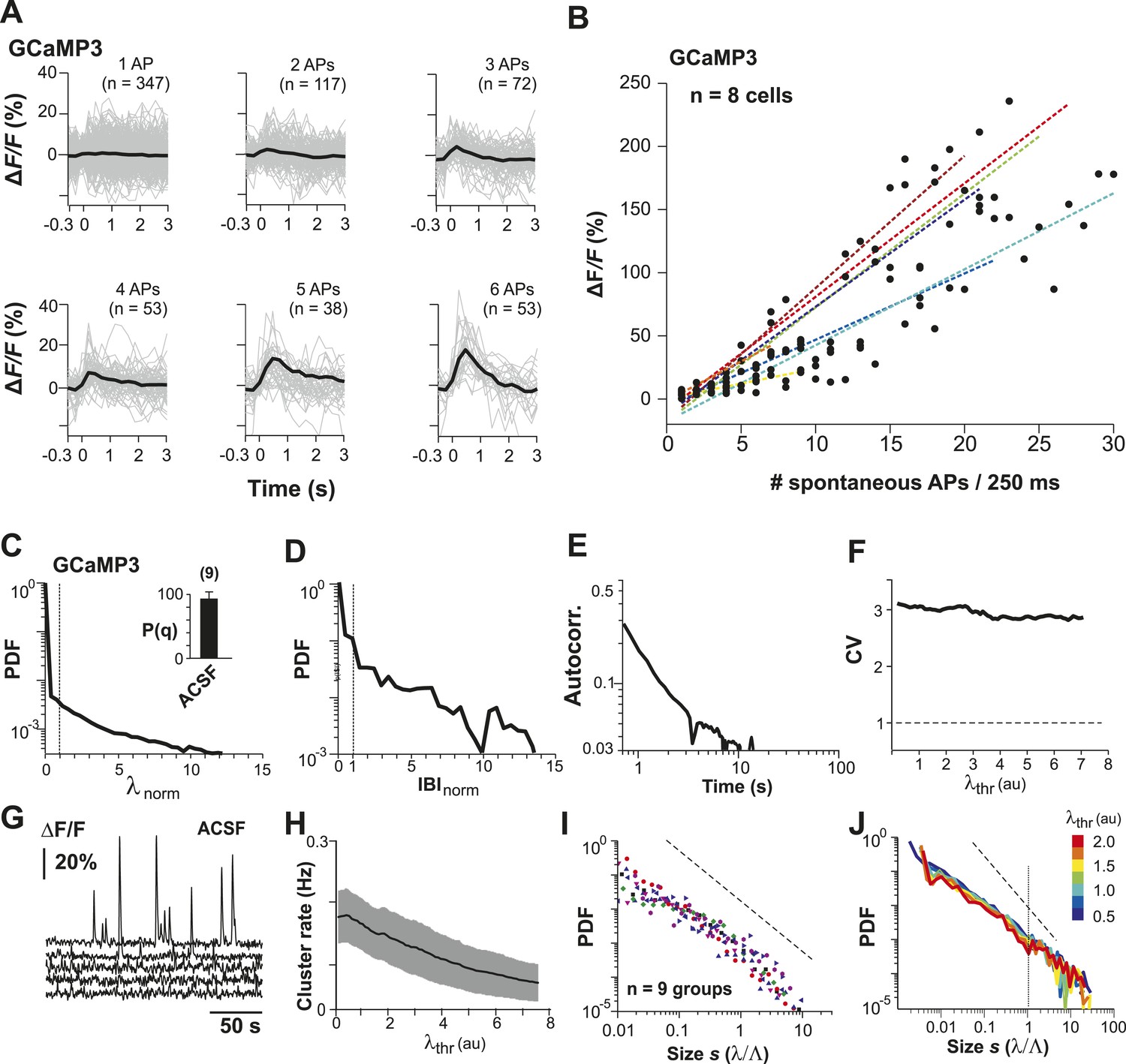
Neuronal avalanche dynamics recorded in vitro using GCaMP3 in organotypic cortex cultures.
(A) GCaMP3 covers a wide dynamic range of spike bursts but fails to reliably capture burst sizes <3 APs. Loose-patch recordings combined with 2-PI of cortex slice cultures grown for ∼2 weeks. Fluorescence traces triggered on spontaneously occurring AP bursts and sorted by the number of spontaneous APs/250 ms. Note the relative insensitivity of GCaMP3 to small bursts establishing a natural threshold of λthr in the data acquisition. Single PN. (B) Summary of change in fluorescent intensity ΔF/F, which increases linearly with spontaneous APs/250 ms, but is undetectably low at sizes <3 APs (n = 8 cells; color codes). Broken lines: regression for individual neurons. (C) Average λnorm distribution for all ROIs. Vertical line, λnorm = 1. (D) Corresponding average distribution in normalized quiescent time intervals, IBInorm. Vertical line, IBInorm = 1. (E) Mean λ autocorrelation function. Note the strong decay in autocorrelation demonstrating temporal correlations for up to 10 s. (F) CV in AP firing is much larger than 1 and independent of λthr. (G) Representative traces of changes in fluorescent intensity (ΔF/F) simultaneously recorded over time from GCaMP3-expressing L2/3 PNs in vitro. Note the relatively sparse activity compared to YC2.60 recordings and large fluctuations in burst amplitudes. (H) Cluster rate as a function of λthr. (I) Cluster size distributions of individual cultures based on GCaMP3 recordings. (J) Average power-law distributions in normalized cluster size s for different λthr (color scale). Observed cascade sizes with the burst indicator GCaMP3 also follow a power law up to the cut-off of s = 1. Dashed line, slope = −1.5.
Author response image 1
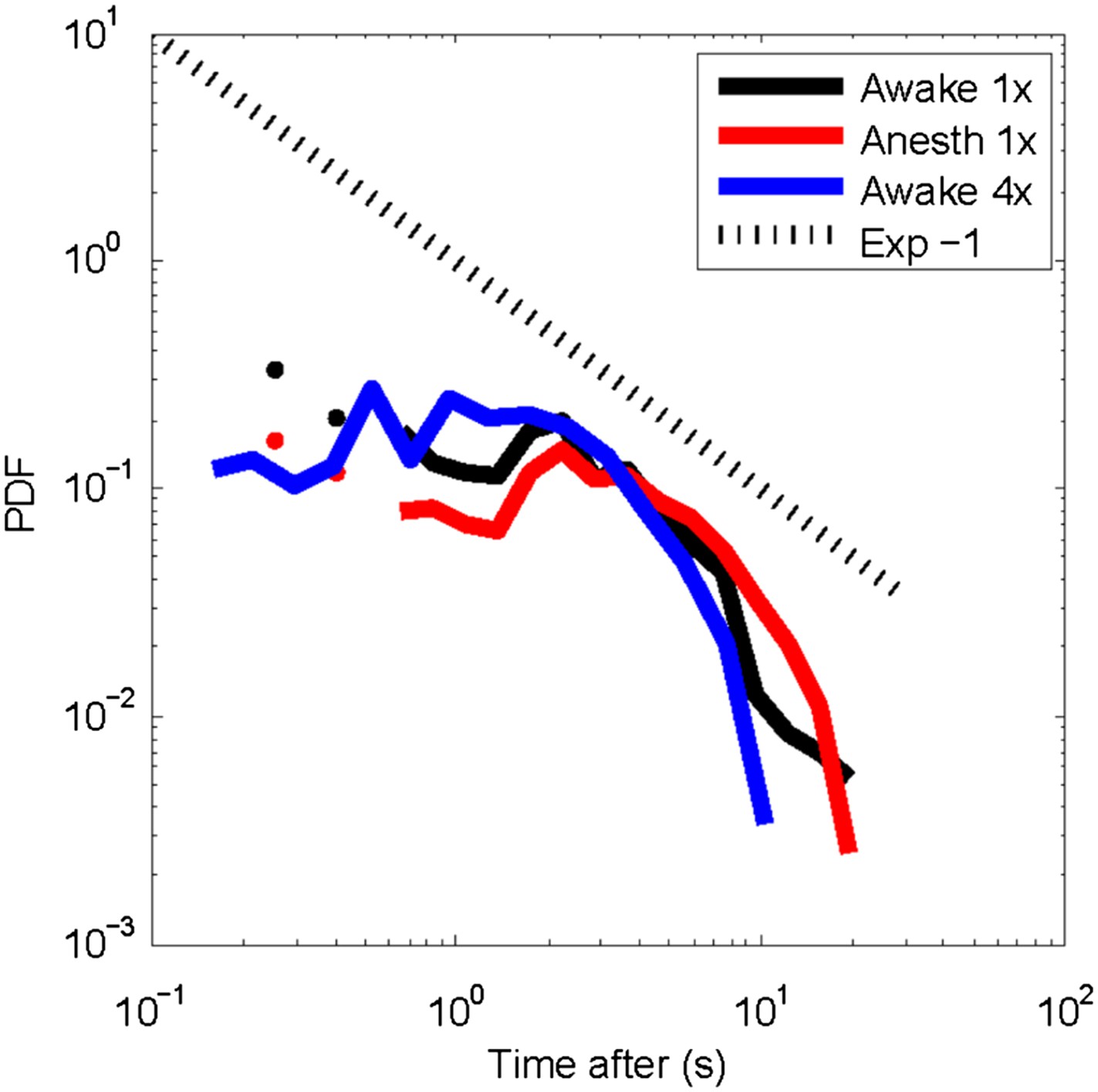
Post-event time histogram of cluster occurrence after occurrence of a large cluster.
In general, large clusters are followed by cluster activity for about 10 s (average over all recordings for each state). Temporal resolution: 1x = 250 ms; 4x ∼88 ms. No significant differences were observed for clusters activity following large clusters between the awake or the anesthetized state.
Author response image 2

Acutely disconnecting of the VTA does not affect neuronal avalanche dynamics in the cortical part of the co-culture.
(a) Light microscopic picture of a cortex (Ctx)-Ventral Tegmental Area (VTA) co-culture grown on a planar microelectrode array (MEA). Left: before acute dissection. Right: after acute dissection of the connection between the two tissue regions (broken line). (b) Spontaneous gamma-burst in the LFP from a single electrode in the cortex part of the culture before and after the dissection. (c) Cluster size distribution before and after dissection (average from 3 cultures). Note that in this plot the probability of cluster size s, i.e. P, is multiplied by s^alpha which translates the power law into a horizontal graph up to the cut-off.
Download links
A two-part list of links to download the article, or parts of the article, in various formats.
Downloads (link to download the article as PDF)
Open citations (links to open the citations from this article in various online reference manager services)
Cite this article (links to download the citations from this article in formats compatible with various reference manager tools)
Irregular spiking of pyramidal neurons organizes as scale-invariant neuronal avalanches in the awake state
eLife 4:e07224.
https://doi.org/10.7554/eLife.07224


