The number of olfactory stimuli that humans can discriminate is still unknown
- Arizona State University, United States
- Bates College, United States
Figures
Figure 1 with 1 supplement
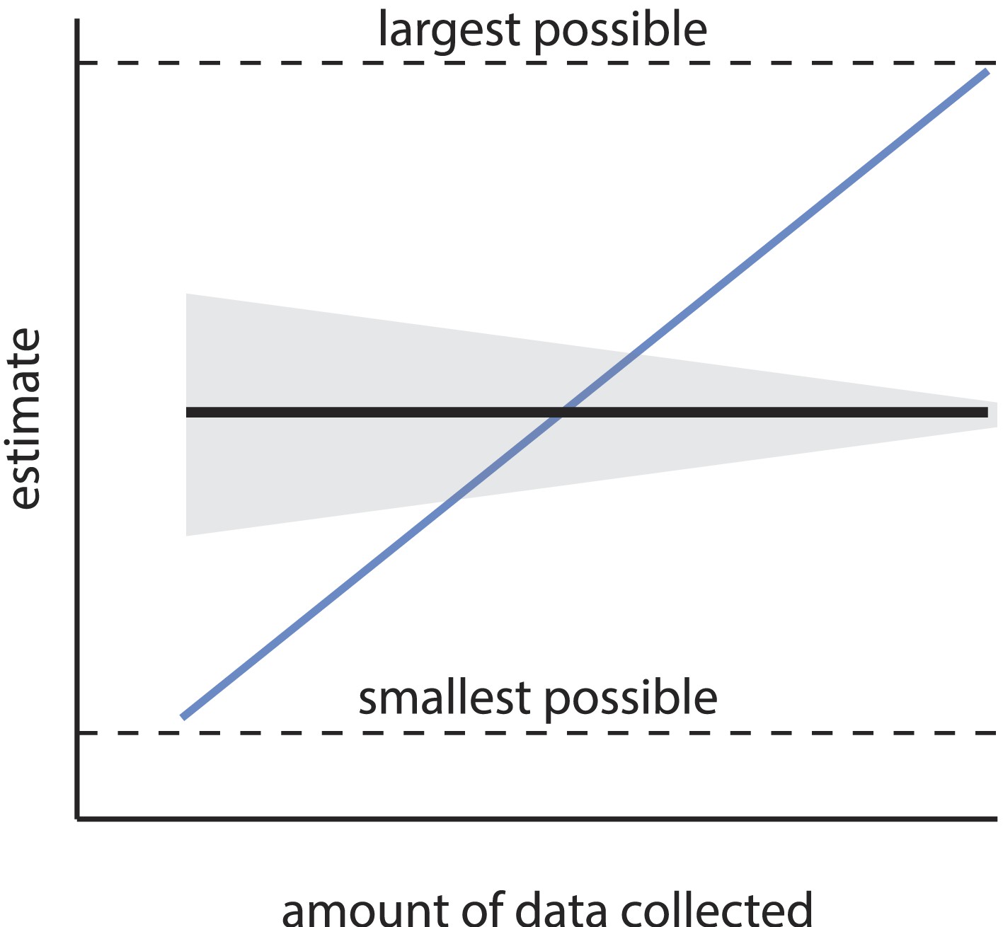
Consistency of an estimator.
An estimator is consistent if the resulting estimate asymptotically converges (in expectation) as sample size increases (black line). Uncertainty in the estimate (gray area) may shrink with sample size, but the estimate itself should not systematically change with sample size, and should converge on the truth. Estimators without this property are termed inconsistent (the blue line is a relevant example), and are considered unreliable, as the resulting estimate can be heavily biased by the sample size. If the estimate has a minimum and maximum allowed value (see Equation 1), an especially inconsistent estimator can even produce any estimate within that range.
Figure 1—figure supplement 1
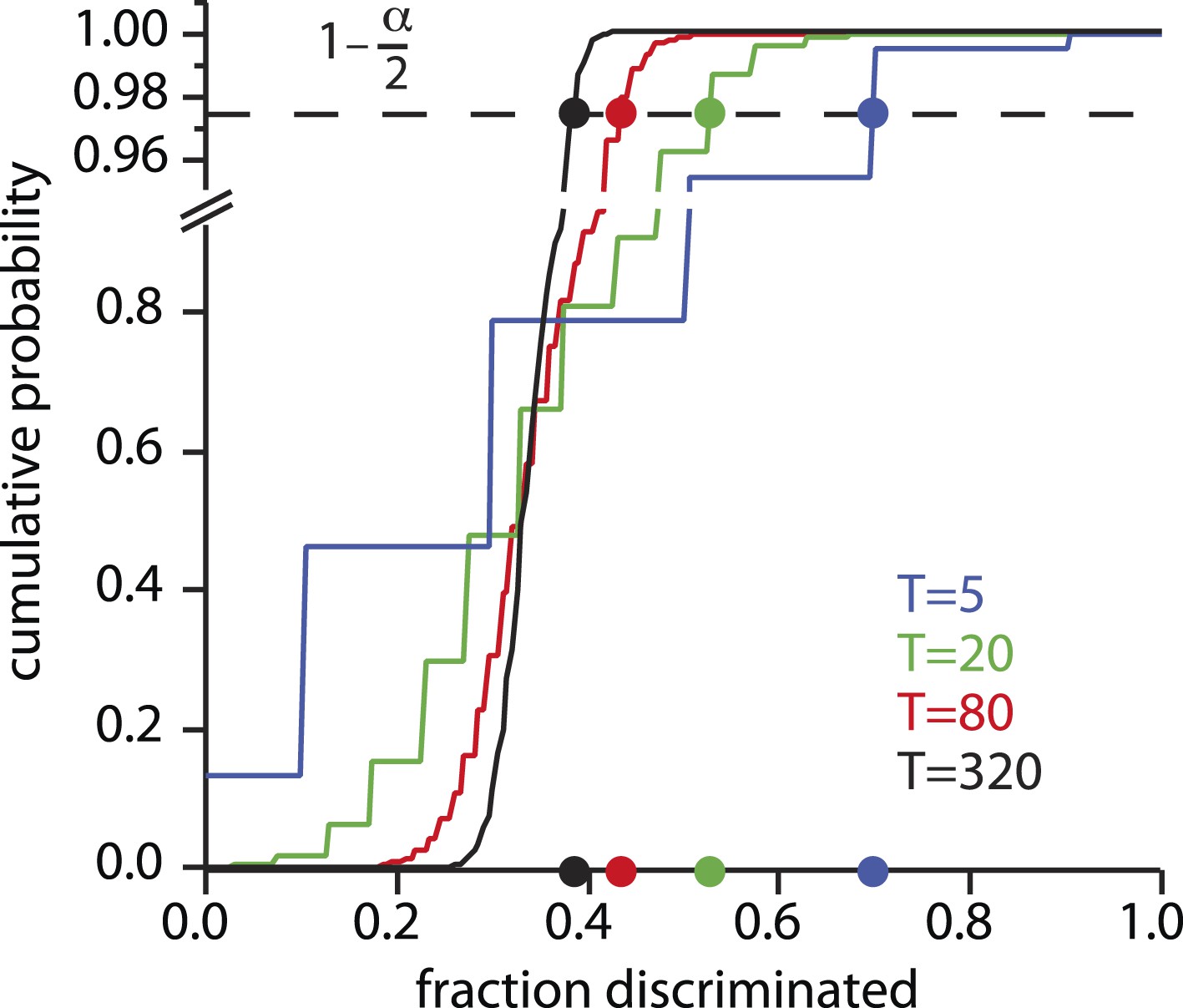
Fraction discriminated at which statistical significance is reached.
For each possible value of the number of tests T conducted per mixture class, there is a cumulative distribution of the fraction f of those tests that will be correctly discriminated, under the null hypothesis of chance responding. The choice of significance threshold α determines the fraction correct required to reject the null hypothesis, and thus count as ‘significantly discriminating’ in the framework. For a given value of α (0.05 shown here, and used in [Bushdid et al., 2014]), the fraction correctly discriminated required to reach this threshold varies greatly with T. Rejecting the null hypothesis can thus be very easy or very hard depending on T (or the number of subjects S, not shown), or on α.
Figure 2 with 1 supplement

Reproduction of the main result published in (Bushdid et al., 2014), from analysis of raw data made available in supplemental materials of (Bushdid et al., 2014).
Compare to Figures 3, 4 in that publication. (A): Discriminability vs mixture overlap, expressed as a percentage of the mixture size N. From this analysis, (Bushdid et al., 2014) derives (vertical dashed line) as the critical value of mixture overlap at which 50% of mixtures achieve ‘significant discriminability’. (B): Estimated number of discriminable mixtures z vs mixture overlap (expressed as a percentage of N) allowing discrimination. The plot is obtained by regression and interpolation of results in A combined with Equation 1, with colors corresponding to values of N as shown in A. For a value of as derived in A, one obtains the ‘trillions’ figure reported in (Bushdid et al., 2014).
Figure 2—figure supplement 1
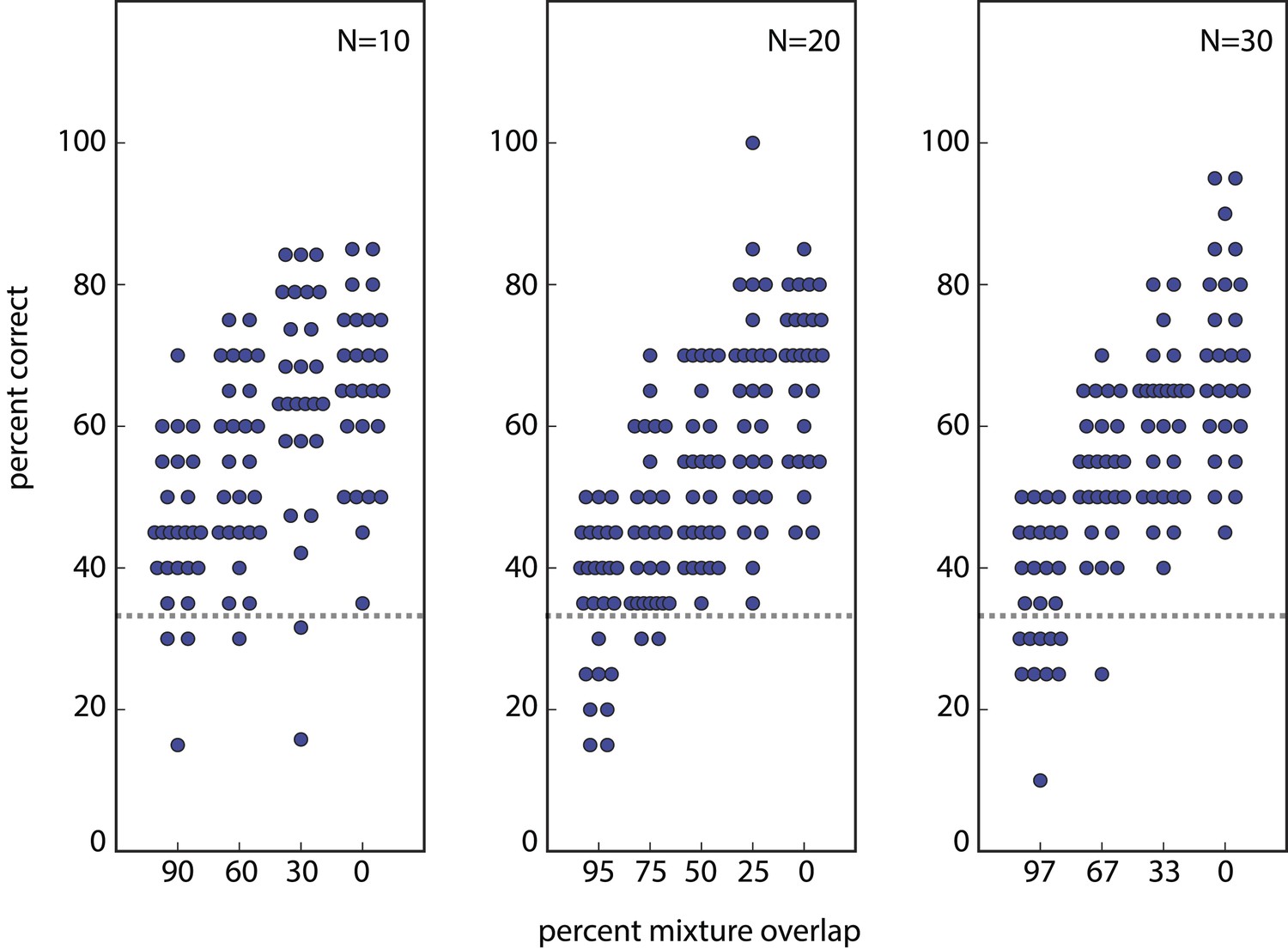
Reconstruction of percent correctly discriminated using raw data from (Bushdid et al., 2014).
This reproduces Figure 2B from (Bushdid et al., 2014), and can be subsequently used to reproduce Figure 3A and ultimately Figure 3C from (Bushdid et al., 2014). Similar reconstructions, using alternative parameter choices, were used as basis for the findings presented in Figure 3A here. Analogous reconstructions of Figures 2C, 3B,D from (Bushdid et al., 2014) (not shown) were used to generate Figure 3B here.
Figure 3 with 1 supplement
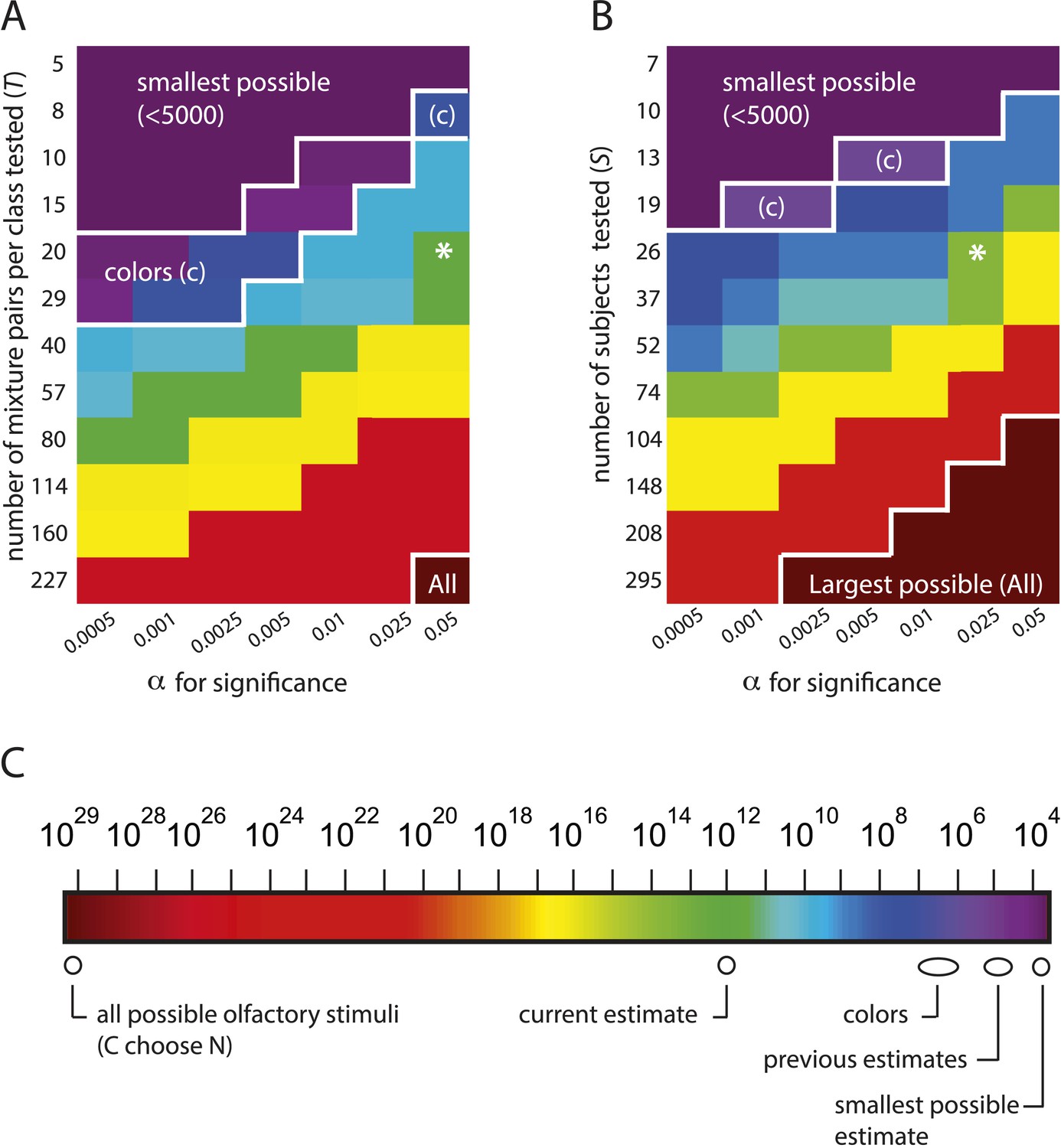
The estimation framework supports nearly any alternative conclusion, including the smallest and largest estimates possible under the framework.
(A): Heat map showing alternative conclusions reached for different choices of T, the number of mixture pairs per class to test, and application of alternative significance threshold α for discriminability, with the data from (Bushdid et al., 2014). Asterisks (*) show the parameter regime (T = 20 mixtures, ) used in (Bushdid et al., 2014). Other values on each axis are chosen in a geometric progression around those parameters. The contour in the lower right labeled ‘All’ demarcates a regime in which one will conclude that the largest possible number of mixture stimuli (i.e., all of them) are discriminable (see Equation 1). The contour in the upper left labeled ‘smallest possible’ demarcates a regime in which one will conclude that the smallest possible number of stimuli are discriminable, that is, only of them. The contour labeled ‘colors’ demarcates a regime in which one concludes that the number of discriminable olfactory stimuli is the same order of magnitude as the number of discriminable colors. (B): Heat map similar to left, only with number of subjects on the vertical axis. A choice of is necessary to obtain the estimate that (Bushdid et al., 2014) reports for this analysis. (C): Colorscale for A and B, with reference landmarks.
Figure 3—figure supplement 1
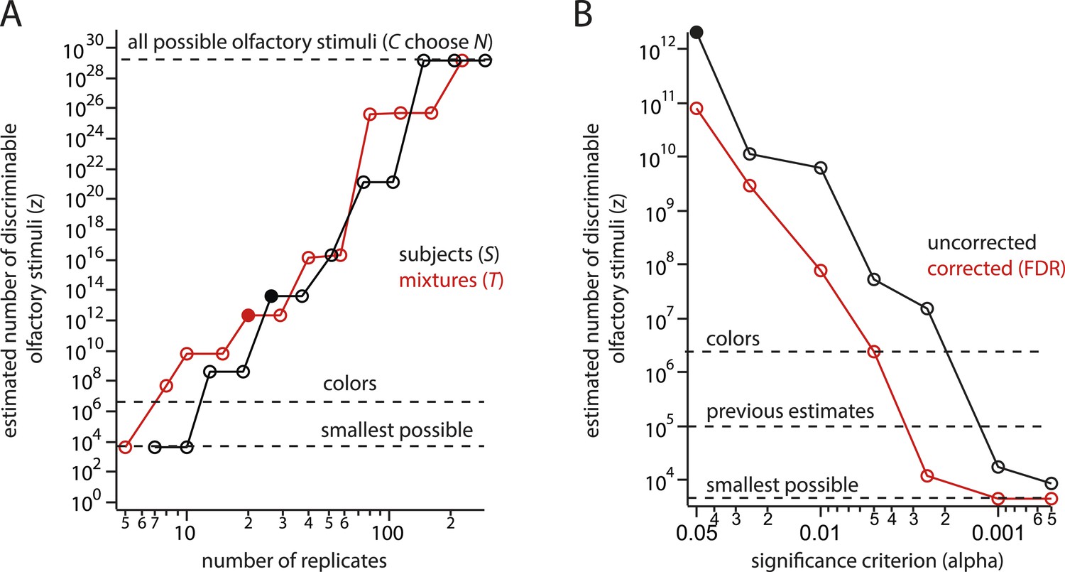
Steep, systematic, and non-asymptotic dependence of the estimate on sample size (S or T) and threshold α for statistical significance.
(A) Dependence of the estimate (for mixtures of N = 30) on sample size. Black shows dependence on the number of subjects S enrolled in the study, Red shows dependence on the number of mixtures T tested per mixture class. Once the number of mixtures or subjects tested is (by no means an unusually large sample size), the conclusion that all possible mixtures are discriminable is guaranteed, in contradiction with experimental results. (B) Dependence of the estimate on the significance threshold α with (red) and without (black) a correction for multiple comparisons. (Bushdid et al., 2014) did not correct for multiple comparisons.
Figure 4 with 2 supplements
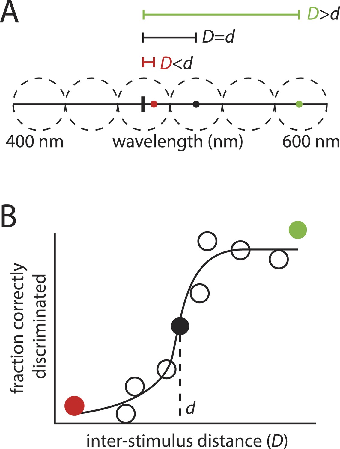
‘Sphere packing' to estimate the number of discriminable colors: the motivation behind the framework in (Bushdid et al., 2014).
(A): Hypothetical example showing a range of visible wavelengths. Relative to a reference stimulus (thick vertical tick mark), extremely distant stimuli (green circle) in this space are easy to discriminate, whereas extremely close stimuli (red circle) may be impossible to discriminate, as they are beyond the resolution of color vision. At some critical inter-stimulus distance, d, stimuli will be ‘just discriminable’ (black circle). A typical stimulus pair on the space, separated by distance D, will tend to be discriminable if , and indiscriminable if . (B): This partitioning into discriminable and indiscriminable sets is captured in the sigmoidal shape of the psychometric curve plotting discriminability vs distance. Knowing that an interval of length d on the space will tend to span ‘just discriminable’ stimuli, one can calculate how many such intervals, z, can be ‘packed’ onto the space to estimate the number of discriminable colors.
Figure 4—figure supplement 1
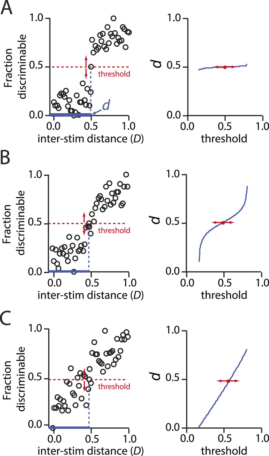
Behavior of psychometric curves for hypothetical data describing discriminability vs inter-stimulus distance.
(A): Left, A sharply sigmoidal relationship in which discriminability changes dramatically and categorically at a critical inter-stimulus distance, d. In all panels, d is the value of the inter-stimulus distance D at which a threshold fraction of stimulus pairs are discriminable. In the left panels, this threshold is set at 0.5. Right, The resulting value of d is nearly invariant to the choice of threshold. (B): Same as above, only for a less sharply sigmoidal data set. There is still a narrow regime in which d is largely invariant to choice of threshold. (C): Same as above, only for a weakly sigmoidal data set. Here, there is no principled means for choosing the d that is characteristic of discriminability relationships for stimuli. The data in C do not support an interpretation in which there is defensible characteristic ‘length scale’ for inter-stimulus distances.
Figure 4—figure supplement 2
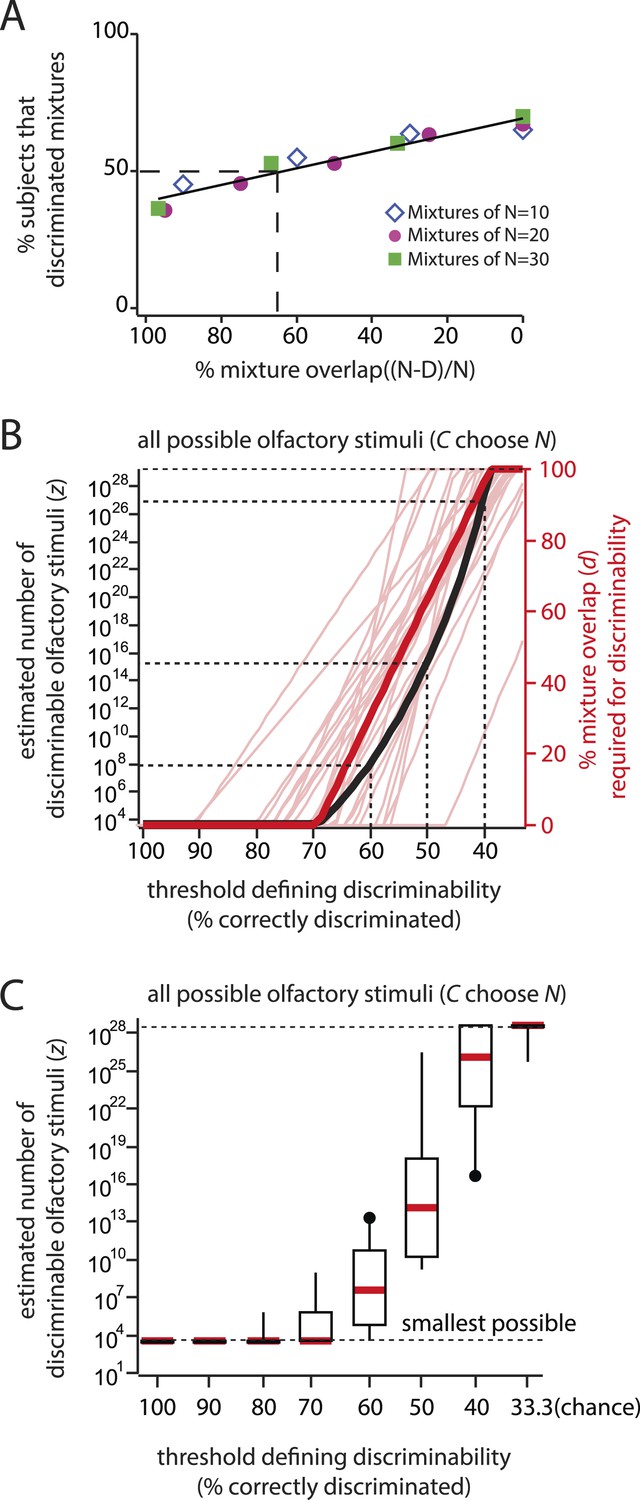
Can the fraction discriminated be used to measure d directly, without resorting to hypothesis testing?
(A): To explore this possibility, the fraction discriminated vs percent mixture overlap is plotted here. This is analogous to Figure 2, except plotting fraction discriminated directly (as in Figure 4—figure supplement 1), instead of fraction significantly discriminable. The threshold (50%) and the procedure for computing mixture overlap at that threshold are as in Figure 2A. Derived from data in (Bushdid et al., 2014) as for Figure 2. (B): The thick red line shows the critical distance d that would result from the data in (Bushdid et al., 2014) for a range of ‘fraction discriminated’ thresholds between 100% (perfect discrimination), and 33.3% (chance discrimination). The curve was obtained by regression on plots like that in Figure 4—figure supplement 2, by analogy to Figure 2 and (Bushdid et al., 2014). Note that d exhibits a nearly constant-slope relationship with threshold, meaning the data are not defined by a characteristic length scale, much like in Figure 4—figure supplement 1C. The thick black curve shows the relationship between z and the chosen threshold. This relationship was obtained directly from d, using Equation 1, as in (Bushdid et al., 2014). The thin red lines correspond to the same calculation for d but using data for only a single subject (one per line), showing similar sensitivity to the choice of threshold. The absence of a robust d for any individual subject argues that the group data are not simply explained by averaging across a population with well-defined, but diverse values of d. Note that very modest and reasonable alternative choices for the threshold result in extremely disparate estimates. The vertical axis is bounded by the smallest and largest possible number of discriminable stimuli allowed by the framework. The dashed lines are a visual guide to specific (threshold, z) pairs. (C): Box and whisker plots showing the median and inter-quartile range for z when restricting the analysis to individual subjects. Note that the worst performing subjects under one threshold can discriminate many more stimuli than the best performing subjects under a slightly more liberal threshold (compare best subject using a 60% threshold vs worst subject using a 40% threshold). Therefore, it is impossible to report with any confidence the number of discriminable stimuli using this approach. In the main text, we show that the actual framework used in (Bushdid et al., 2014) is nominally employed to make a more principled choice of threshold; however it merely cloaks the arbitrariness of the threshold choice, but does not eliminate it.
Figure 5
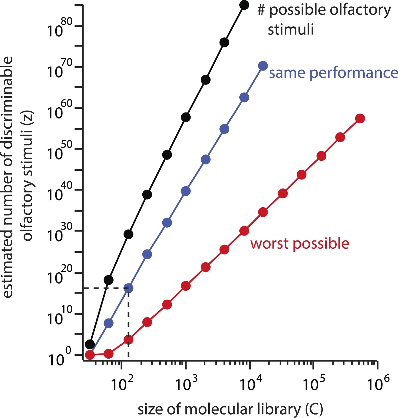
Explosive growth of the estimate z on the size (C) of the molecular library.
The number of possible stimuli z that can be assembled by choosing N = 30distinct molecules from a library of size C increases geometrically with C (black line). If a library of a different size had been used, and similar subject performance resulted, the estimated number of discriminable stimuli z would grow along a similar trajectory (blue line). Even if performance deteriorated as C increased, the estimate could never fall below the red line, which represents worst-case performance (d = N). This results from the combinatorial explosion inherent in Equation 1.
Figure 6

Upper and lower bounds of the number of discriminable stimuli.
(A): Number of discriminable olfactory stimuli as a function of the estimated difference limen (the fractional mixture overlap allowing discrimination). This is simply the behavior of Equation 1 as a function of d, for the three values of N used in (Bushdid et al., 2014); the red dot (in both A and C) corresponds to the value reported in (Bushdid et al., 2014). The smallest possible estimate (thousands of stimuli) is indicated by the dotted line running the length of the abscissa (note also the y-intercept). As described in the text and in the supplement, this graph in fact shows the behavior of the upper bound (the so-called Hamming bound) for the mathematical problem of sphere packing. Compare with Figure 3D in (Bushdid et al., 2014). (B): Same plot as in A, only using the lower-bound for the same calculation. (C): Upper and lower bounds of the sphere packing problem for the N = 30case (green lines from A and B, respectively. The dark gray bar shows the range of defensible estimates under the sphere-packing framework, using the d calculated in (Bushdid et al., 2014). Using that d, the number of discriminable stimuli may be as small as ∼10,000, and is guaranteed to be no larger than ∼1 trillion. Since the estimate of d is also fragile (Figure 3), the data may in fact support any value in the shaded gray area.
Tables
Table 1
Definitions of parameters
| z | Estimated number of discriminable olfactory stimuli |
| C | Number of distinct compounds available to make mixtures |
| N | Number of distinct compounds in a mixture |
| O | Number of distinct compounds shared by a mixture pair |
| D | Number of distinct compounds in one mixture of a pair that are not shared by the other. |
| class | All mixture pairs with the same value of N and D. |
| d | The value of D for which mixture pairs of a given N are more likely than not to be discriminable at a rate significantly above chance. |
Table 2
Estimates of z, the number of discriminable olfactory stimuli, for different possible parameters values, for the C = 128, N = 30 case used in (Bushdid et al., 2014)
| A | ||
|---|---|---|
| # Discriminable stimuli (z) | Significance threshold (α) | # Tests per class (T) |
| 0.05* | 20* | |
| † | 0.05* | 5 |
| ‡ | 0.05* | 185 |
| 0.001 | 20* | |
| 0.01 | 15 | |
| B | ||
|---|---|---|
| # Discriminable stimuli (z) | Significance threshold (α) | # Subjects (S) |
| 0.025* | 26* | |
| † | 0.025* | 7 |
| ‡ | 0.025* | 135 |
| 0.001 | 26* | |
| 0.01 | 15 | |
-
This recapitulates selected points from Figure 3.
-
* Indicates that the parameter value was used in (Bushdid et al., 2014). We assume here that new subjects perform similarly to the original subjects.
-
Note that (†) and (‡) are the smallest and largest possible values allowed by the framework from (Bushdid et al., 2014).
Download links
A two-part list of links to download the article, or parts of the article, in various formats.
Downloads (link to download the article as PDF)
Open citations (links to open the citations from this article in various online reference manager services)
Cite this article (links to download the citations from this article in formats compatible with various reference manager tools)
The number of olfactory stimuli that humans can discriminate is still unknown
eLife 4:e08127.
https://doi.org/10.7554/eLife.08127


