Synchronized amplification of local information transmission by peripheral retinal input
- Stanford University School of Medicine, United States
Figures
Figure 1
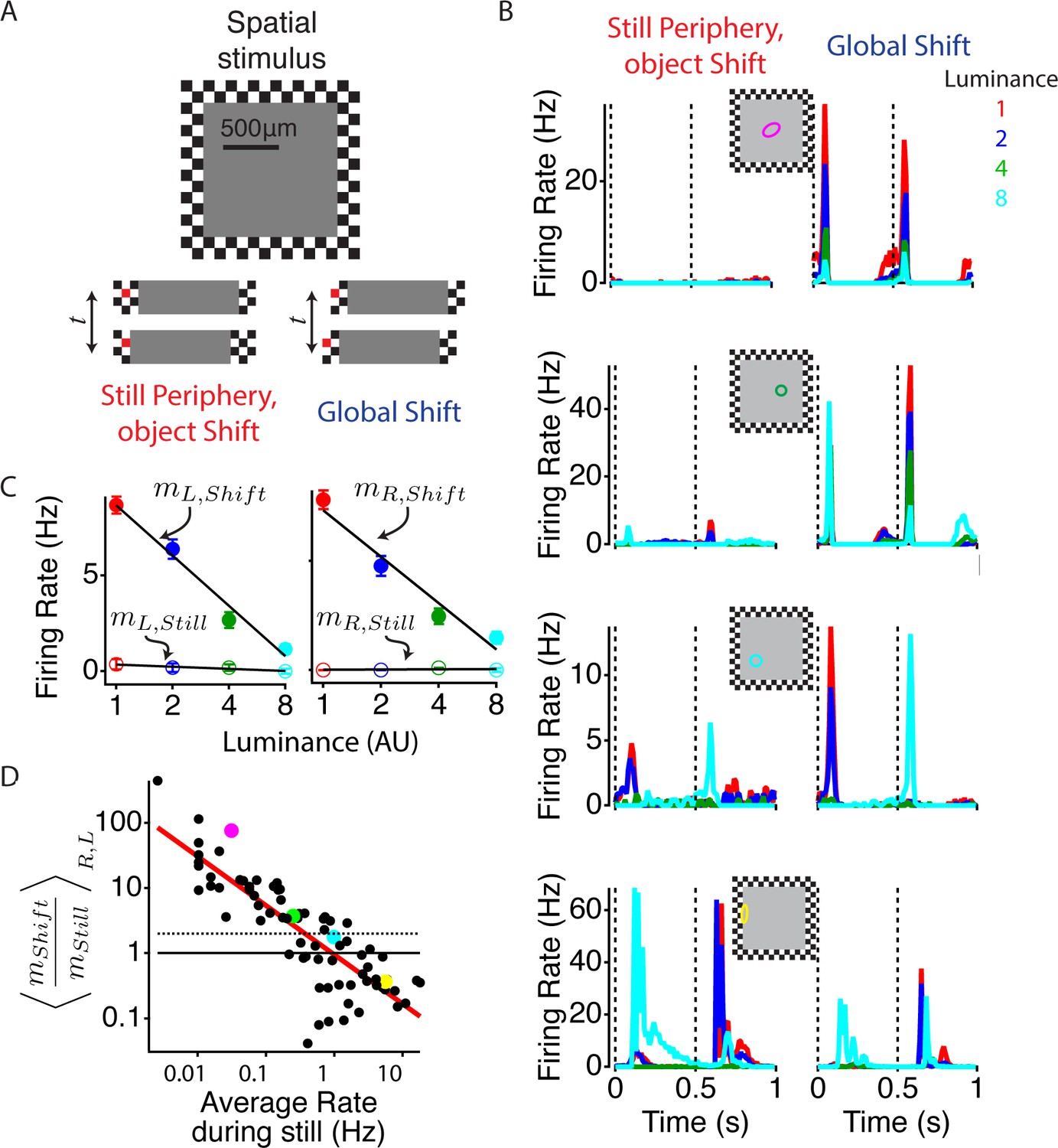
Global image shifts increase sensitivity to weak local input.
(A) (Top) A diagram of the stimulus is shown. The central square representing an object shifted left or right either in the presence of a static periphery (still periphery, moving object, left in bottom panel) or in conjunction with the periphery (global shift, right in bottom panel). In both conditions, the central stimulation was the same. Shifts occurred every 0.5 s, and the luminance level in the object changed every 110 s to one of four values spaced logarithmically. Lower panel shows the central stimulus region under both peripheral conditions. One checker is colored red (not used in actual stimulus) to help the reader identify the relationship between this particular checker and the central stimulus. (B) Average firing rate response of four different cells from different preparations to four different luminance values under both peripheral conditions: object shift (left), global shift (right). Stimulus shifts to the right (0 s) and left (0.5 s) are marked with dotted lines. The classical (linear) receptive field center, computed from a white noise checkerboard stimulus is shown as a colored oval. (C) Average firing rate computed between 50 and 150 ms after the stimulus shifted to the left and right for the cell shown in (B, top panel), colors of dots show different luminance levels corresponding to the curves in (B). A linear fit (lines) to the data was used to compute the sensitivity m to the luminance of the central region, computed as the slope of the firing rate vs. the log of the central luminance for left and right object shifts with periphery still (open circles, , ) and for global shifts (filled circles, ). (D) The ratio of the luminance sensitivity m during global and object shifts compared for each cell to the firing rate in the object shift condition, indicating the strength of the object shift stimulus. Axes are logarithmic. Results for and were averaged over shifts to the left and right. Cells above the dotted line increased the slope of firing vs. central luminance by more than a factor of two during a global shift compared with an object shift. Colored dots correspond to the cells shown in (B).
Figure 2 with 1 supplement
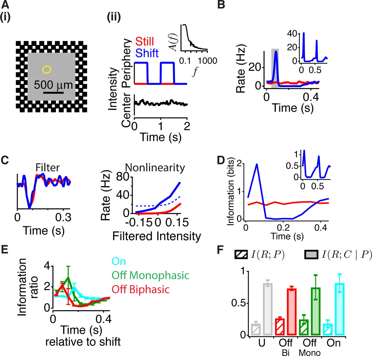
Peripheral gating of information transmission.
(A-i) Spatial stimulus design showing central and peripheral regions. (A-ii) The temporal sequence in each region. The center stimulus flickered randomly with a naturalistic amplitude spectrum proportional to 1/f (inset). In the periphery, the stimulus either shifted (reversed in sign) every 0.5 s or was still. Most cells had linear receptive field centers fully contained in the central region (yellow oval indicates receptive field center). (B) Peristimulus time histogram aligned to the time of peripheral stimulation. Inset shows the two different peripheral shifts averaged separately, indicating that both excitation and inhibition occur for both peripheral phases. (C) Filters and nonlinearities of a linear-nonlinear model computed from the spike times and the center signal. In the Shift case, only spikes from the high firing rate window were used (gray box in B). The dashed nonlinearity is the curve that would have resulted from a vertical shift of the Still case to account for the observed increase in activity in the high firing rate window. (D) Mutual information between the spike count in a 50 ms time window and the central region as a function of time after the peripheral shift. Inset shows information computed separately for left and right shifts of the grating. (E) Average for different cell types of the normalized information in the Shift condition for three different cell types; biphasic Off (n = 95 cells), slow Off (n = 10) and slow On (n = 7). Information was normalized by the value in the last bin. (F) Average across cells of the information that the spike count carries about the peripheral signal I(R; P) or about the central region once information about peripheral input has been removed (see Materials and methods). By the chain rule of mutual information, the two quantities add to the total amount of information the spike count conveys about the stimulus, I(R; P, C).
Figure 2—figure supplement 1
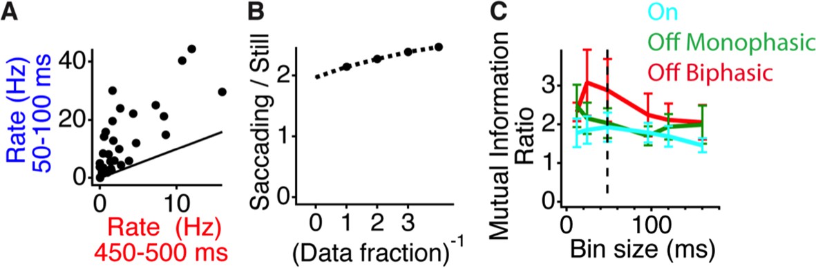
Peripheral shift increases the response to central stimuli with a natural temporal spectrum.
(A) Scatter plot of the firing rate for each cell during gating (50–100 ms) and baseline (450–500 ms) time windows. (B) Stability of information calculations over the amount of data size. The increase in the information ratio in the gating window (Figure 2) was computed for all of the data, and various inverse fractions shown on the horizontal axis. A second-order polynomial fit was used to extrapolate the curve to the limit of infinite data (Strong and Koberle, 1998). (C) Ratio between the mutual information in the gating window and the information in the last time window right before peripheral excitation as a function of the bin size used for counting spikes. Shown are values for On cells, monophasic Off cells and Biphasic Off cells. Dotted line represents bin size used in Figure 2.
Figure 3 with 1 supplement
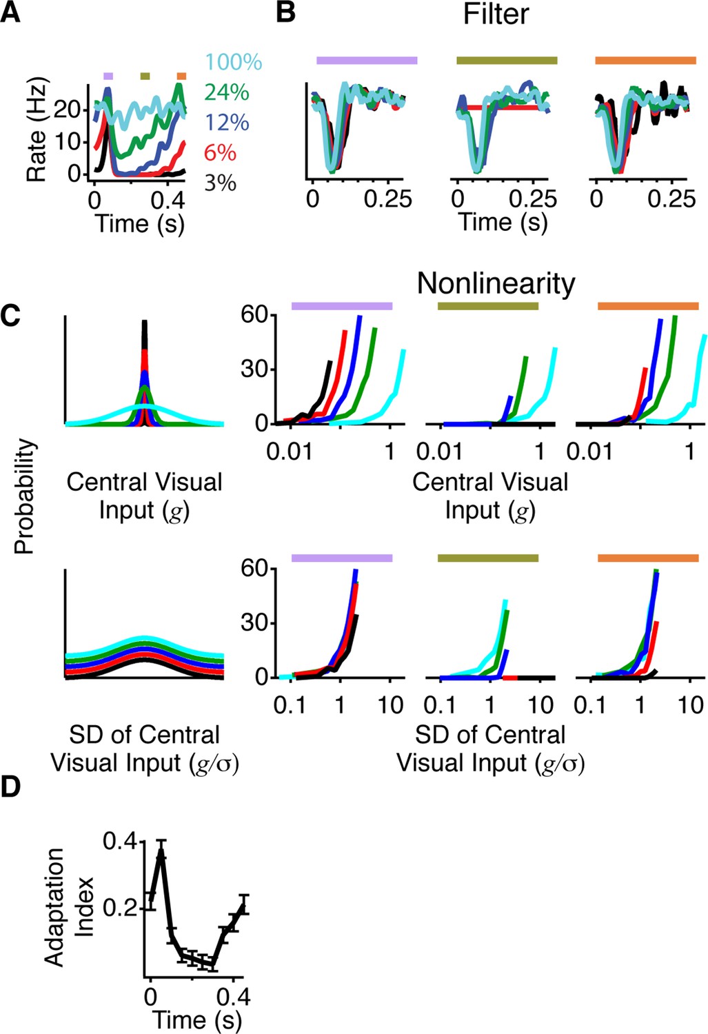
A more adapted representation underlies an increase in information transmission.
(A) The spatial stimulus was the same as in Figure 2. The time course of the central stimulus was a Gaussian white noise stimulus with one of four different contrasts or 100% binary contrast, consisting of black and white intensity values. PSTHs are shown for the different conditions. (B) Filters computed using only spikes from 50 ms time windows, corresponding to color boxes in (A). Purple, gating window; Olive green, suppression window; Orange, recovery window. (C) Input distributions (left) and nonlinearities in the same three 50 ms time windows as in (B). Upper curves are all in units of the linear prediction; lower curves show the same data but in units of standard deviation of the linear prediction. The abscissa is displayed on a logarithmic scale, such that normalization by the standard deviation produces a lateral shift. (D) Average adaptation index across cells that exhibited peripheral excitation (see Materials and methods, n = 400).
Figure 3—figure supplement 1
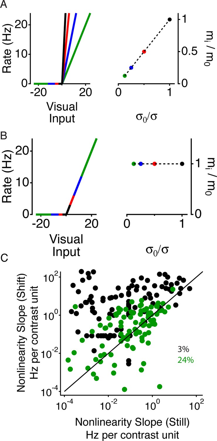
Periphery induced changes in adaptation.
(A) Left, schematic nonlinearities for a hypothetical perfectly adapted cell, where the slope of the nonlinear is inversely proportional to the contrast. Right, normalized slope of the nonlinearities vs. normalized inverse contrast, showing the two quantities should be equal for an ideally adapting cell. (B) Same as (A) for a non-adapting cell, showing that for a non-adapting cell the slope does not change. (C) Average nonlinearity slope during the 50 ms time window corresponding to just after the peripheral shift (purple in Figure 3B–D) vs. the average nonlinearity slope during the 50 ms corresponding to the recovery time window (orange) for both high (24%) and low (3%) contrast in the center region.
Figure 4 with 1 supplement
Different stimulus properties are conveyed with different dynamics.
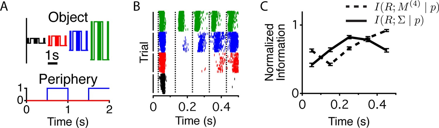
(A) Experimental design for the measurement of sequence and contrast information. The center object follows a binary M-sequence at four different contrasts. Each position in the sequence and contrast combination occurs at all possible times relative to a peripheral shift. (B) Raster plots for an example cell aligned to the time of the peripheral shift and ordered according to contrast. Many different sequences are shown for each contrast value. Luminance values in the center change every 100 ms, generating temporally discrete responses. Vertical lines show the times used to extract responses for the information calculation. (C) Average across cells (n = 94) of the normalized information conveyed about the contrast (four different levels, solid line) or the four frame stimulus sequence M(4) (dashed line) as a function of time since the shift.
Figure 4—figure supplement 1
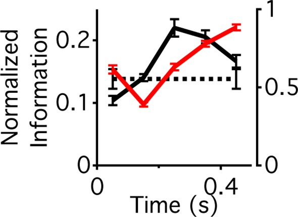
Different components of the stimulus are conveyed with different dynamics.
Information that the response carries about the contrast at a particular time relative to peripheral stimulation (solid black trace, left vertical axis) and information that the response carries about the center sequence M(4) given that the response occurs at a given contrast and time relative to peripheral stimulation (red trace, right vertical axis). These two terms sum to the total information given by the response about the stimulus at a given time relative to peripheral stimulation, . Information that the response carries about the time, p relative to peripheral stimulation, (dotted black trace, left axis). Although this quantity is a number and not a function of time, it is shown here for comparison.
Figure 5 with 1 supplement
Gating of information through a shift in an internal threshold.
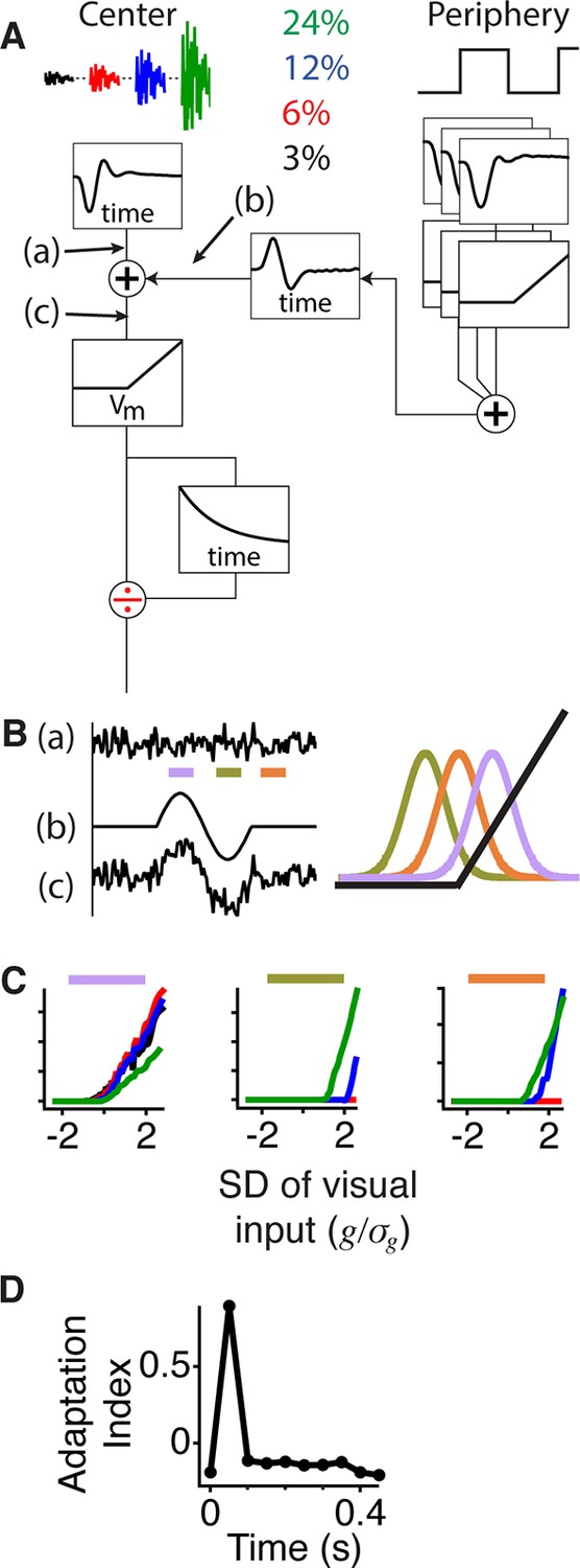
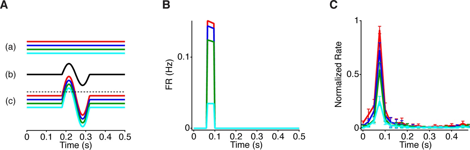
(A) Model of a cell where two pathways are combined prior to a threshold and an adaptive block, implemented here as a feed forward divisive effect with a memory. Peripheral pathway is composed of many nonlinear subunits making the pathway insensitive to the stimulus spatial pattern and delivers biphasic input to the central pathway (first positive, then negative). The stimulus is Gaussian white noise at 3–24% contrast matching the experiment (and colors) in Figure 3. The central pathway is composed of a linear temporal filter, because stimulus is only a function of time. (B) Signals arising at points (a), (b) and (c) whose locations in the model are marked in panel (A). When the peripheral input is positive (gating window, purple bar) or negative (suppression window, olive green bar) the central input is shifted to higher or lower values with respect to the baseline state (recovery window, orange bar) and fixed threshold. Right, the Gaussian distribution of the filtered stimulus occurring at point (c) in (A) compared to the threshold nonlinearity occurring after point (c) in (A) during the gating (purple), suppression (olive green) and recovery (orange) windows. The peripheral input effectively shifts the Gaussian mean with respect to the fixed threshold. (C) Model responses to the same Gaussian stimulus used in Figure 3 at the times of the corresponding color bars in (B). (D) Adaptation index for the model’s output as a function of time after the shift.
Figure 5—figure supplement 1
Model responses to peripheral gating for steady central stimuli.
(A) Traces show the signals at points (a–c) indicated in the model in Figure 5A. Different steady intensity levels from the center (a) are summed with dynamic peripheral input (b) to generate distinct transient responses in the model (c) prior to the threshold. Dotted line represents the cell’s threshold, which is only crossed with the aid of peripheral excitation. (B) PSTHs generated by the model when constant luminance levels are delivered to the model. (C) Average PSTH (n = 21 cells) of the firing rate produced by a central 1 mm square at one of four constant luminance levels logarithmically spaced, with the periphery shifting every 0.5 s. In contrast to Figure 1, the central square is fixed in space and does not move with the periphery. Error bars are SEM.
Figure 6 with 1 supplement
Similar spatial scale for peripheral excitation and inhibition.
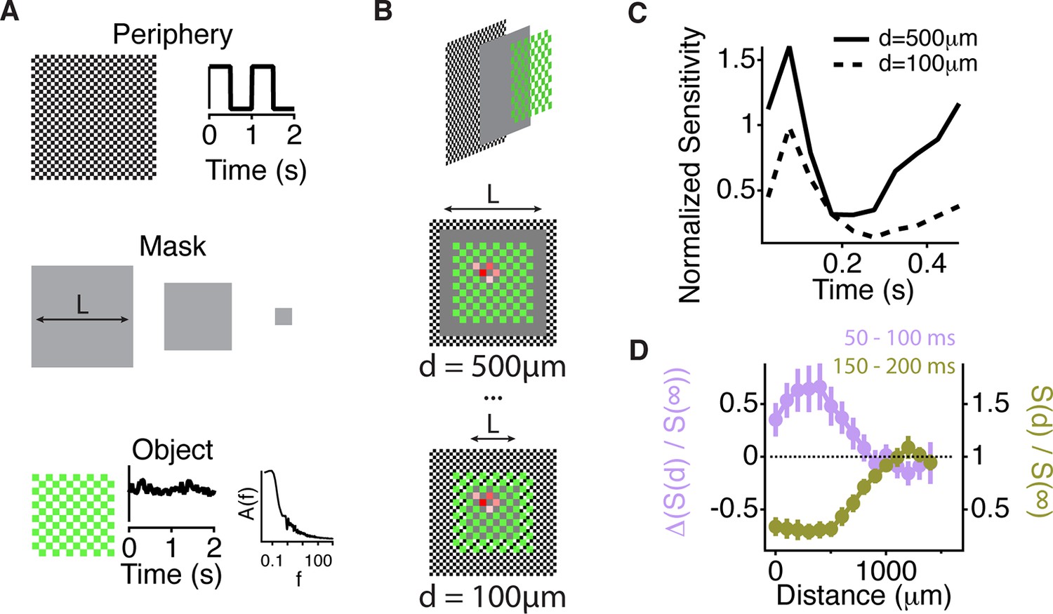
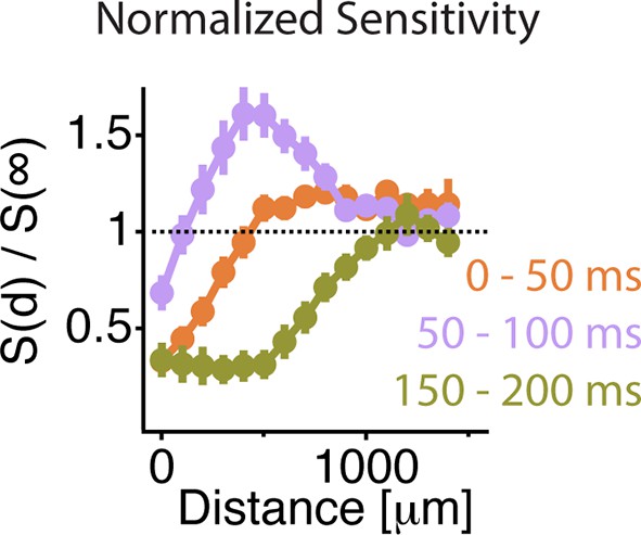
(A) Experimental design for measuring the spatial scale of peripheral excitation and inhibition (see Materials and methods). (Top) The periphery was a checkerboard pattern with squares of 50 μm covering all the screen that reversed in intensity at 1 Hz. (Middle) A gray mask with no temporal component and variable size, L, was drawn on top of the checkers. (Bottom) The object was a checkered pattern with a square size of 100 μm (shown in green for illustration). Object squares in the center flickered with a pink noise distribution, with an equivalent contrast of 10% , changing every 30 ms. (B) Top, schematic of how the different components of the stimulus were layered. Middle and Bottom, a sample cell’s spatial receptive field for the object stimulus is shown in red with the color representing sensitivity to that particular square of the object for two different sizes of the intermediate mask. With this design, the object does not change across the different conditions and any change in the sensitivity to the object is due to the distance of the peripheral checkers. (C) Average over cells (n = 66) of the normalized sensitivity to the object stimulus, which was computed as the average slope of the nonlinearity of a linear-nonlinear model normalized by the average slope of the nonlinearity when the background was at infinity, as a function of time bin t, relative to the background shift for two different mask sizes. (D) Average of the normalized sensitivity as in panel (C) as a function of distance between the cell and the mask during the gating window (50–100 ms after the shift) and an inhibitory window (150–200 ms after the shift). Each point in a line corresponds to the minimum distance between the cell’s linear receptive field and the background checkers for a particular background condition mask L. For the gating window, the baseline of sensitivity at 0–50 ms, which is too soon after the shift to be affected by it, was subtracted for each distance d. This subtraction was not done for the recovery window because at distances less than 500 µm, residual inhibition creates a saturating decrease in sensitivity, causing many cells to have zero slope at this time. See Figure 6—Figure supplement 1 for sensitivity before the subtraction of this baseline.
Figure 6—figure supplement 1
Similar spatial scale for peripheral excitation and inhibition.
Average normalized sensitivity as in Figure 6D as a function of distance between the cell and the mask during three different time windows. At 0–50 ms, the sensitivity had not yet recovered from the previous shift. Therefore, the sensitivity at 0–50 ms was taken as a baseline, which was subtracted from the sensitivity at 50–100 ms, as shown in Figure 6D.
Figure 7 with 2 supplements
Model of central information for natural scenes with eye movements.
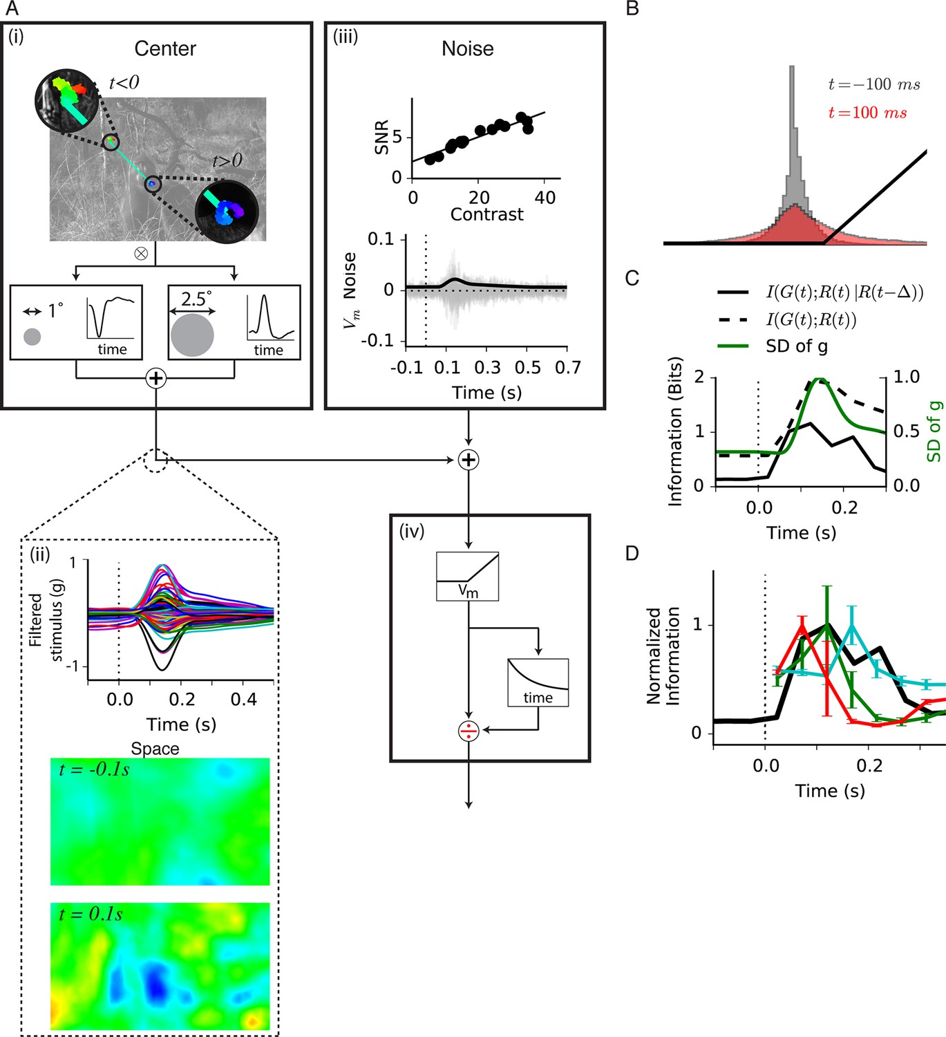
(A) Spatiotemporal model used in the simulation. (A-i) An eye movement trajectory overlaid on a natural image, consisting of fixational drift, and a sudden eye movement (green line) that takes the center of each cell from one image location (insets) to another. The image series is convolved (⊗) with a separable spatiotemporal filter previously measured from a fast Off-type bipolar cell (Baccus et al., 2008), yielding a linear prediction for a bipolar cell at each spatial location. (A-ii) (Top) The linear prediction for 100 model bipolar cells over different images as a function of time. A sudden eye movement occurs at 0 s (dotted line). Vertical scale is in arbitrary units. (Middle and Bottom) The linear prediction is shown for a population of bipolar cells (one at each spatial location) at 100 ms before and after the sudden image shift responding to the image and eye movement trajectory shown in (A-i). Color scale is the same in both images. (A-iii) Noise model. (Top) signal to noise ratio measured experimentally in a bipolar cell from repeats of a spatially uniform Gaussian white-noise stimulus under different stimulus contrasts (Figure 7—figure supplement 1) (Ozuysal, 2012). (Bottom) Noise generated with this model, shown in the same arbitrary units as in (A-ii) Top. Black line is the standard deviation of the noise at each point in time. (A-iv) (Top) After the linear central input is summed with the noise, the result is passed through a rectifying nonlinearity and then through a feedforward divisive operation representing a simplified version of adaptation, as in the model in Figure 5. (B) Distributions of linear prediction values over many images at different times, compared with the rectifying nonlinearity (black line) from (A-iv). Distributions before t = 0 s and after 350 ms are identical. (C) Dynamics of information transmission after a sudden eye movement. The Shannon mutual information between the linearly filtered stimulus, , and the model output, (black dashed line) at a given delay from the shift, p, and the conditional mutual information between the same quantities when conditioning on the response at a previous time (black solid line). Both stimuli and responses were averages over bins of 50 ms. Also shown is the standard deviation of the linear prediction from (A-iii) (green line). (D) Comparison of the expected conditional mutual information from the model at each time after an image shift (black line) with the time course of information transmission measured during experiments for several cell types (reproduced from Figure 2E).
Figure 7—figure supplement 1
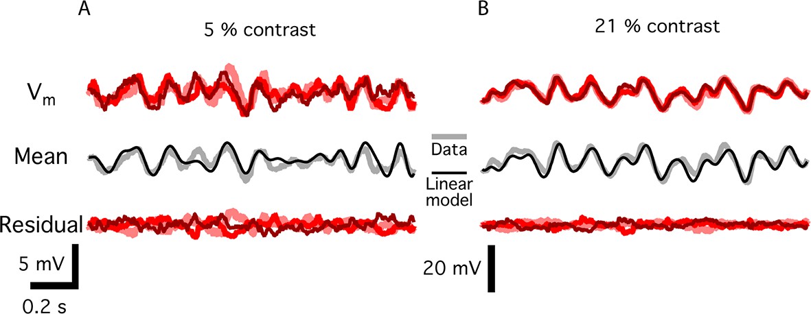
Noise measurements in bipolar cells.
(A) Top. Three membrane potential responses of a fast Off bipolar cell responding to a repeated Gaussian white noise of 5% contrast. Middle. Mean of the three repeats, the standard deviation of which was an estimate of the signal carried by the bipolar cell, along with a linear model of the response, consisting of the stimulus convolved with a linear temporal filter. Bottom, the residual membrane potential, which is the difference between each individual response and the mean value. The standard deviation of these residual responses is estimated to be the noise at each contrast. (B) Same as A. for 21% contrast.
Figure 7—figure supplement 2
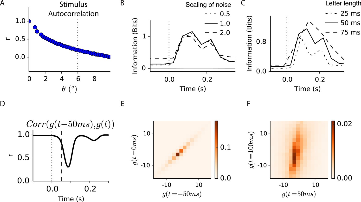
Correlations and information in a spatiotemporal model of gating.
(A) Correlation coefficient between image patches of 1° (the size of the simulated bipolar cell’s center) as a function of their distance. Vertical dotted line shows the sudden eye movement used in the simulation, exceeding most positive correlations between images patches. (B) Conditional mutual information between the filtered stimulus and the output of the spatiotemporal model in Figure 7 at a given delay from the shift, p, at three different noise levels. Doubling or halving the standard deviation of the noise did not change the results qualitatively. Gray trace indicates the near-zero level of information when randomly permuting the response with respect to the filtered stimulus, indicating that the joint distribution of filtered stimulus and response was sampled sufficiently. (C) Same as (B) but changing the bins over which linear predictions and responses are computed. (D) Correlation coefficient between linear prediction samples, and , shown at different times, t. Significant decorrelation is seen even as early as 50 ms after the shift. (E, F) Joint probability distribution of and , at two times separated by 50 ms, showing that prior to a sudden shift in the image linear inputs are highly correlated in time and more decorrelated just after the shift.
Download links
A two-part list of links to download the article, or parts of the article, in various formats.
Downloads (link to download the article as PDF)
Open citations (links to open the citations from this article in various online reference manager services)
Cite this article (links to download the citations from this article in formats compatible with various reference manager tools)
Synchronized amplification of local information transmission by peripheral retinal input
eLife 4:e09266.
https://doi.org/10.7554/eLife.09266


