Fast turnover of genome transcription across evolutionary time exposes entire non-coding DNA to de novo gene emergence
- Max-Planck Institute for Evolutionary Biology, Germany
Figures
Figure 1 with 2 supplements
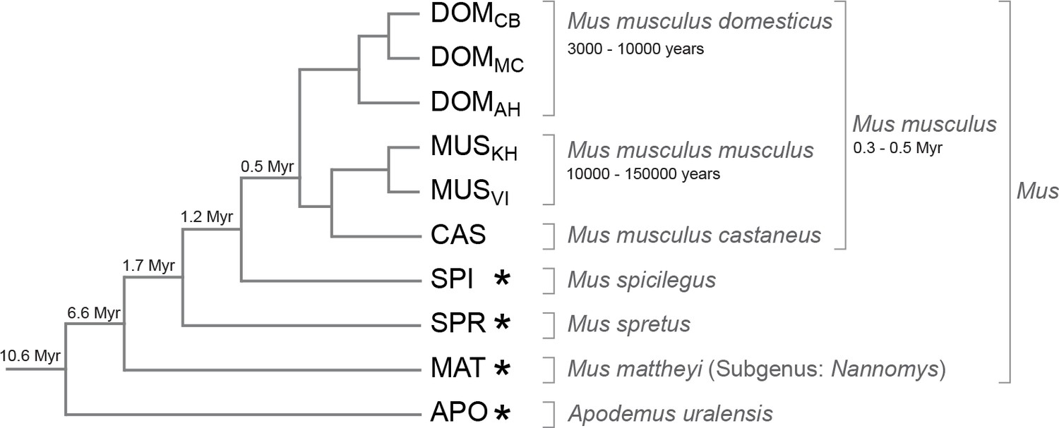
Phylogenetic relationships and time estimates for the taxa used in the study.
New genome sequences were generated for taxa with *. A common genome was constructed across all taxa (Figure 1—figure supplement 1) based on a mapping algorithm that is not affected by the sequence divergence between the samples (Appendix 1). Figure 1—figure supplement 2 shows the intersection of genome coverage between the named species.
Figure 1—figure supplement 1
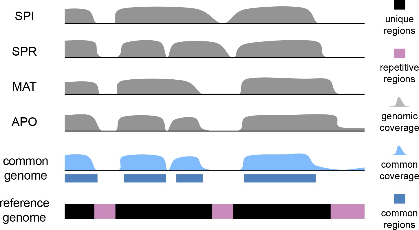
Scheme for the establishment of the 'common genome' using genomic reads and the mouse reference genome.
The common genome represents the portion of the reference which is present and detectable across all species. The genome sequencing, processing and sequence analysis were done in the same way as for transcriptomes, effectively removing possible biases derived from sequencing and mapping. Note that the assignment of the common genome fraction was done after mapping all genomic and transcriptomic reads to the reference, i.e. the mapping process was not affected by a reduced mapping target.
Figure 1—figure supplement 2
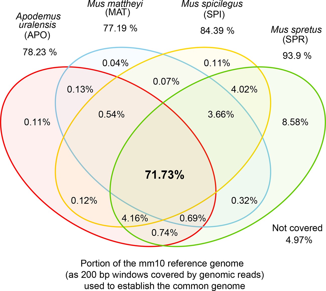
Venn diagrams of representation of the common genome, derived from 200bp windows covered in genomic reads in species with more than one million years divergence to the reference.
Windows covered by all four species are used as the common genome (shown as the intersection of all species).
Figure 2
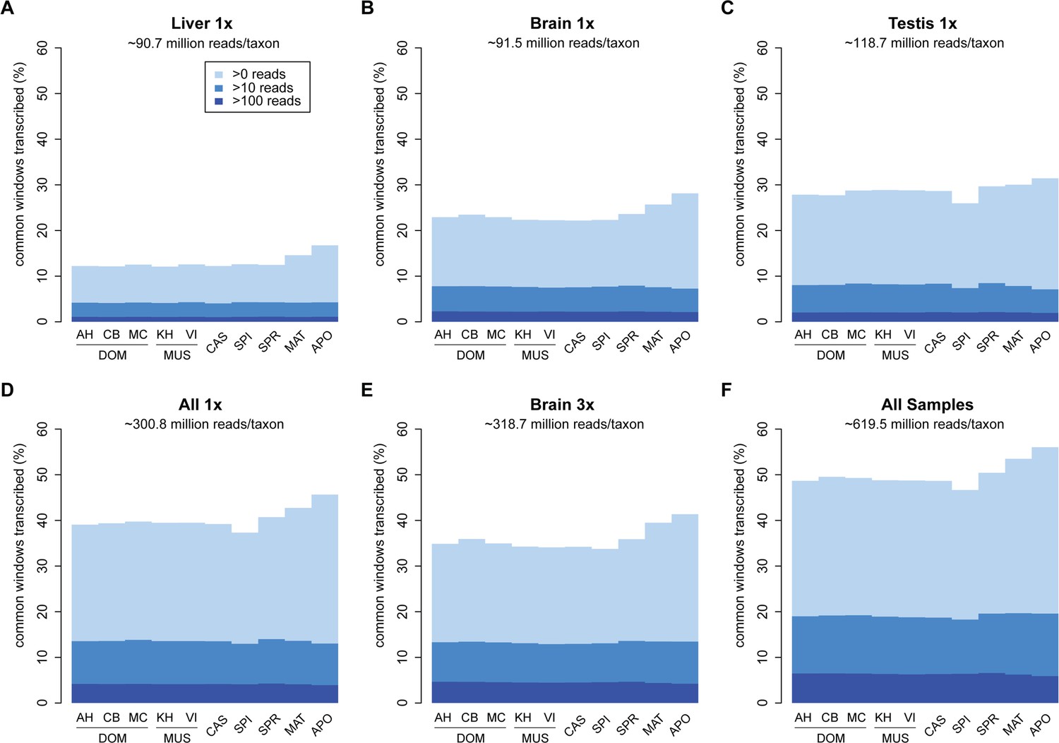
Transcriptome coverage of the common genome per taxon.
(A–C) Liver, brain and testis, respectively, sequenced at approximately the same depth. (D) Combination of samples from A–D. (E) Additional sequencing of brain samples at 3x depth, compared to B. (F) Combination of all samples, including additional brain sequencing. Three coverage levels are represented by colors from light blue to dark blue: window coverage with at least 1, 10 and 100 reads. Taxon abbreviations as summarized in Figure 1, with closest to the reference genome to the left of each panel and most divergent one to the right. Note that the slight rise in low read coverage for the distant taxa could partially be due to slightly more mismapping of reads at this phylogenetic distance (see Appendix 1 for simulation of mapping efficiency), but is also affected by a larger fraction of singleton reads (compare Figure 4—figure supplement 1).
Figure 3 with 2 supplements
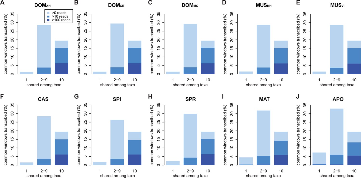
Distribution of shared and non-shared windows with transcripts for each taxon, based on the aggregate dataset across all three tissues.
Three classes are represented: i) windows that are found in a single taxon only, ii) windows found in 2–9 taxa and iii) windows shared among all 10 taxa (from left to right in each panel). Windows with transcripts were first classified as belonging to one of the three classes, independent of their coverage, and were then assigned to the coverage classes represented by the blue shading (from light blue to dark blue: window coverage with at least 1, 10 and 100 reads). Taxon names as summarized in Figure 1. Figure 3—figure supplement 1 shows an extended version where class ii) is separated into each individual group. Relative enrichment of annotated genes in the conserved class is shown in Figure 3—figure supplement 2.
Figure 3—figure supplement 1
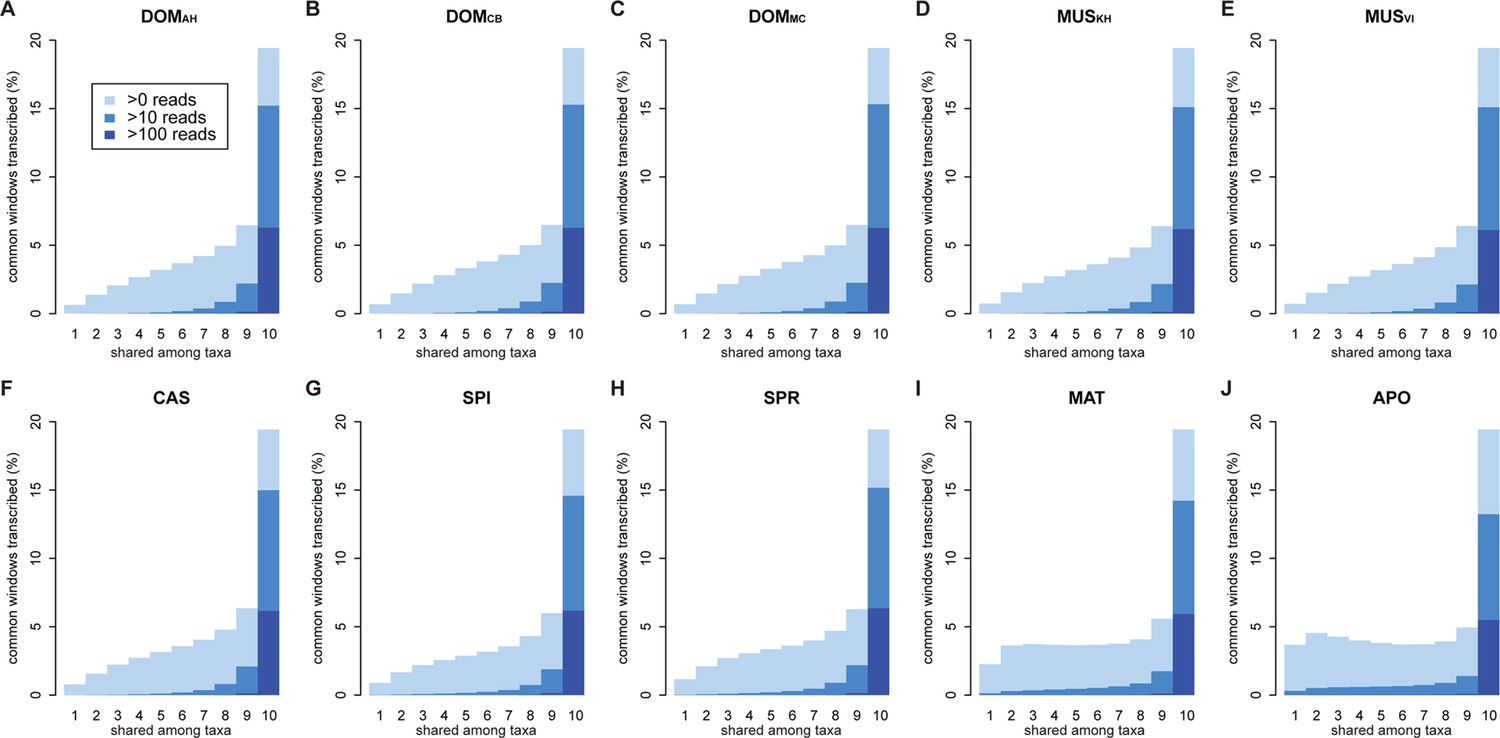
Distribution of shared transcripts according to the number of taxa shared, based on the aggregate dataset across all three tissues.
Windows with transcripts were first classified as belonging to each of the sharing categories (from 1 to 10), independent of their coverage, and were then assigned to the coverage classes represented by the blue shading (from light blue to dark blue: window coverage with at least 1, 10 and 100 transcripts). Taxon names as summarized in Figure 1.
Figure 3—figure supplement 2
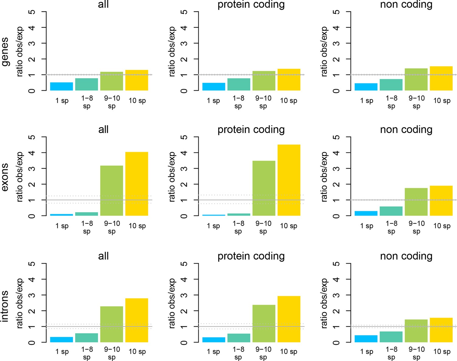
Windows transcribed across most species (9 or more) are strongly enriched in genes known from the reference genome, while windows transcribed in some taxa (8 or less) are strongly depleted from known genes.
The effect is most evident for protein-coding genes, but still present for non-coding genes.
Figure 4 with 3 supplements
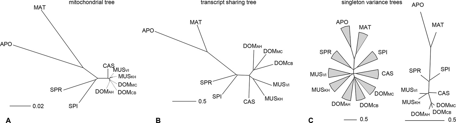
Distance tree comparisons based on molecular and transcriptome sharing data.
(A) Molecular phylogeny based on whole mitochondrial genome sequences as a measure of molecular divergence (black lines represent the branch lengths, dashed lines serve to highlight short branches). (B) Tree based on shared transcriptome coverage of the genome, using correlations of presence and absence of transcription of the common genome. All nodes have bootstrap support values of 70% or more (n = 1000). (C) Tree based on shared transcriptome coverage of singleton reads only from subsampling of the extended brain transcriptomes. Left is the consensus tree with the variance component between samples depicted as triangles, right is the same tree, but only for the branch fraction that is robust to sampling variance. Taxon names as summarized in Figure 1. Figure 4—figure supplement 1 shows the fraction of singletons in dependence of each sample in each taxon, Figure 4—figure supplement 2 in dependence of read depth. Figure 4—figure supplement 3 shows an extended version of the analysis shown in 4C for higher coverage levels.
Figure 4—figure supplement 1

Fraction of windows with singletons (one paired read) of the common genome per taxon.
(A-C) Liver, brain and testis, respectively, sequenced at approximately the same depth. (D) Combination of samples from A–D. (E) Additional sequencing of brain samples at 3x depth, compared to B. (F) Combination of all samples, including additional brain sequencing. Light gray indicates singletons observed in each individual sample/taxon combination. Dark gray indicates singletons across the whole experiment, i.e. not re-detected in any other tissue or taxon. Taxon abbreviations as summarized in Figure 1, with closest to the reference genome to the left of each panel and most divergent one to the right. Note that the rise in singleton number for the distant taxa can be ascribed to the longer branch length, i.e. absence of closely related taxa in which the singleton could have been re-detected.
Figure 4—figure supplement 2
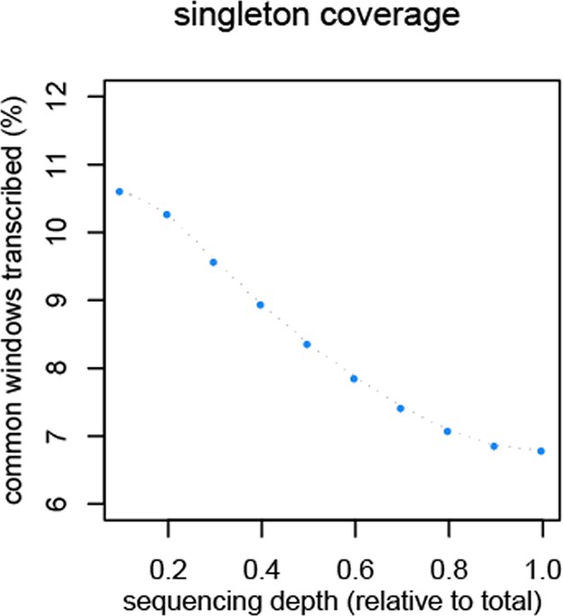
Reduction of singletons in dependence of aggregate sequencing depth.
https://doi.org/10.7554/eLife.09977.012
Figure 4—figure supplement 3
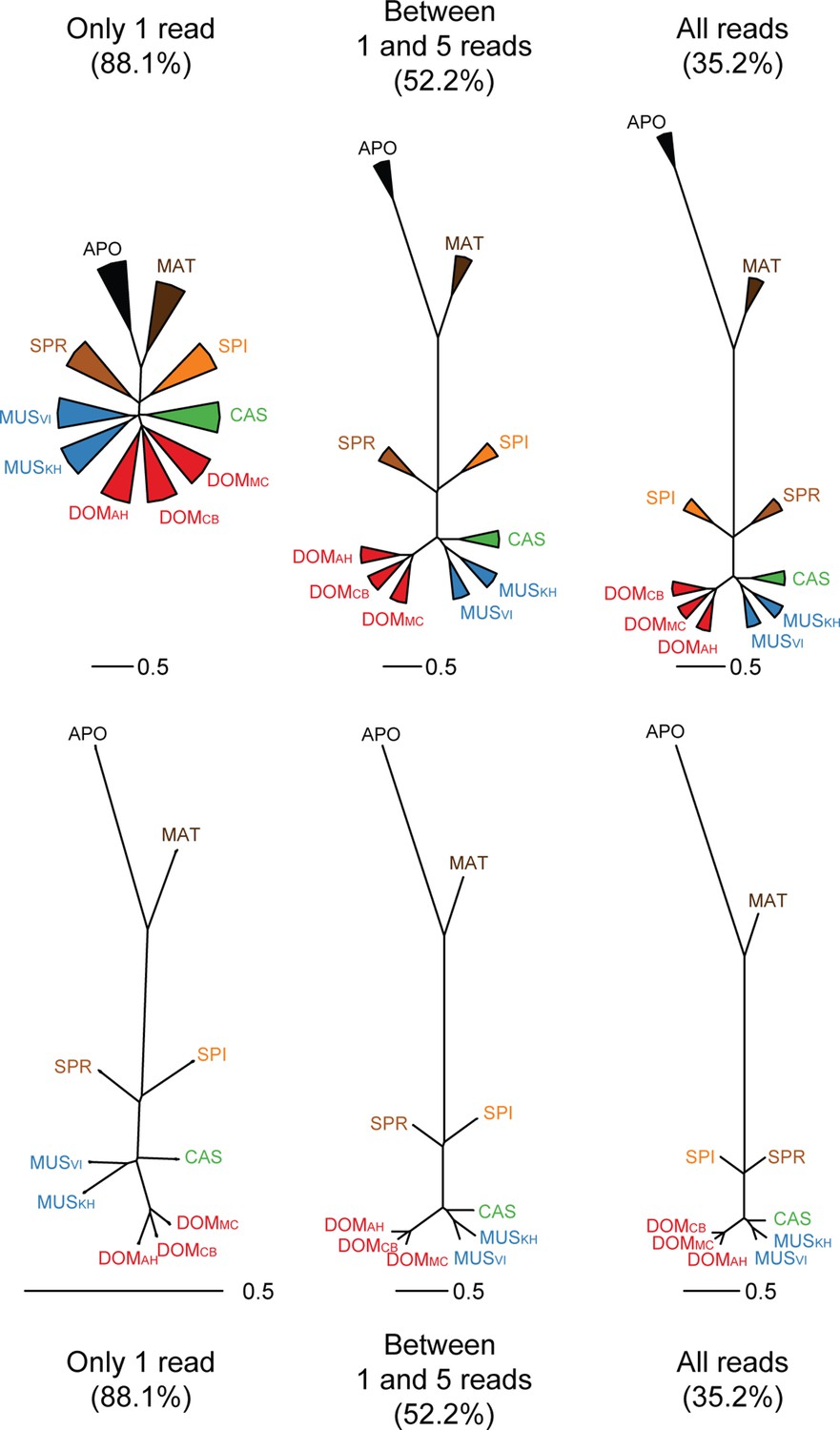
Trees based on shared transcriptome coverage of the genome, using binary correlations.
We used the deep sequenced brain samples to estimate the proportion of sampling artifacts in terminal branches, and effectively subtracted the proportion of artifacts to obtain reliable phylogenetic signals. Each brain sample was split in three completely independent samples of 100 million reads. Top: Trees constructed using: regions covered only with one read in each taxon, regions covered by 1 and 5 reads (very low expression), regions covered by any reads, regions above 10 reads (mid expression) and regions above 100 reads (high expression). The percentage shown indicates the average level of sampling artifacts for each threshold, derived from the length of the terminal branches not found in all replicates of each taxon, i.e. the uncorrelated portion across samples of the same origin. These numbers are highest for the lowly expressed regions, and are lowest for the highly expressed regions, and are more or less constant within comparisons. Once subtracted, the phylogenetic signal remains robust. Taxon names as summarized in Figure 1. The figure part with the 1 read fraction corresponds to Figure 4C.
Figure 5
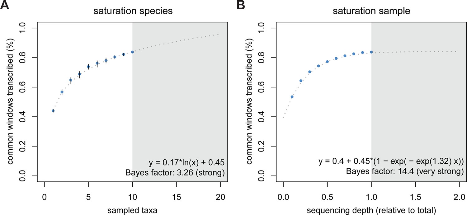
Rarefaction, subsampling and saturation patterns using all available samples and reads.
(A) Sequencing depth saturation as estimated from an increase in the number of taxa. (B) Sequencing depth saturation as estimated from increasing read number. Blue dots indicate increases per sub-sampled sequence fraction or taxon added from our dataset. Gray dotted line indicates the predicted behavior from the indicated regression, and gray area shows the prediction after doubling the current sampling either by additional taxa (A) or in sequencing effort (B). Each analysis was tested for logarithmic and asymptotic models. Best fit was selected from ΔBIC, with Bayes factor shown and qualitative degree of support shown. Standard deviations are shown as black lines in A, and are too small to display in B (note that due to the sampling scheme for this analysis, the values above 50% are not statistically independent and that the 100% value constitutes a single data point without variance measure).
Figure 6
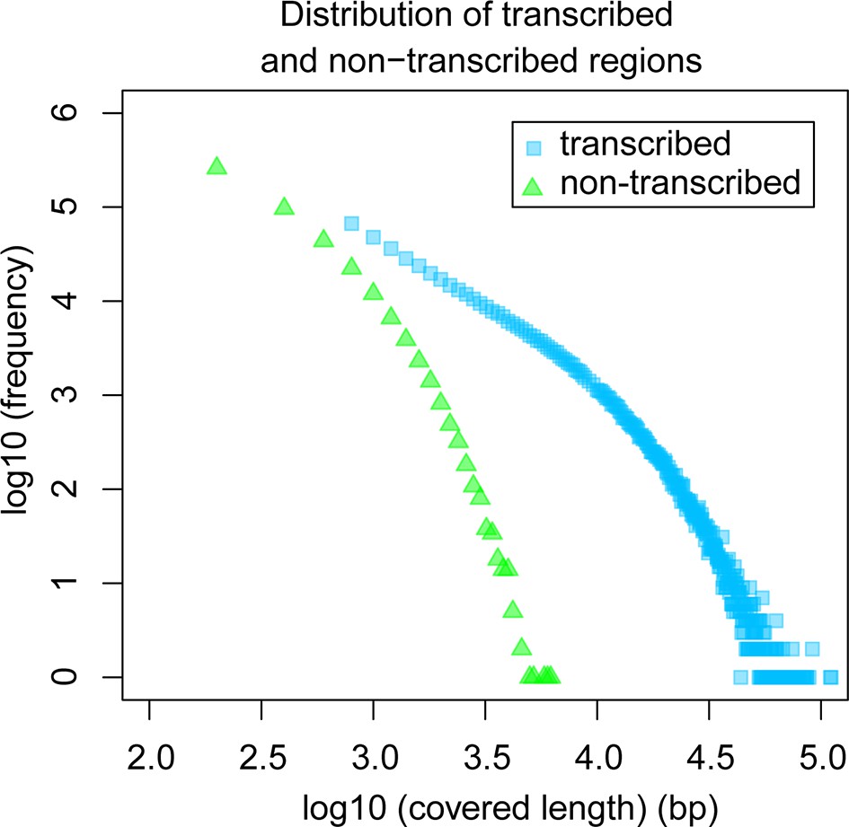
Comparative analysis of lengths of regions transcribed or not transcribed across all data (including deeper brain sequencing) in all samples.
Size distribution of regions not covered in any transcript (green) versus size distribution of regions with at least one transcript (blue).
Appendix 1—figure 1
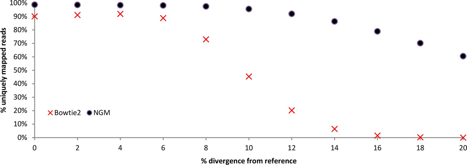
Performance of NextGenMap compared to Bowtie2.
https://doi.org/10.7554/eLife.09977.021
Appendix 1—figure 2
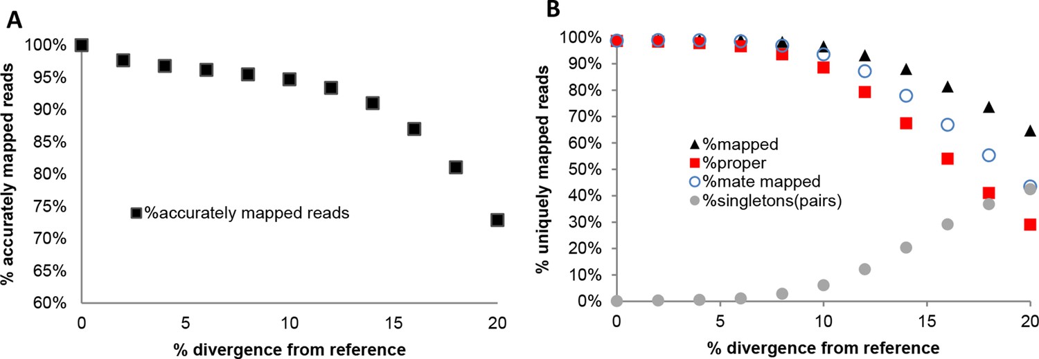
Performance of NextGenMap in terms accuracy of mapping using the same set of reads and increasingly divergent versions of the reference genome (A), and paired-end mapping statistics (B).
https://doi.org/10.7554/eLife.09977.022Tables
Table 1
Genome sequencing and read mapping information relative to the C57Bl/6 reference strain (GRCm38.3/mm10).
| Species | Uniquely mapping reads (MAPQ >25) | Mean coverage depth (window based) | Reference coverage (% windows) | Total sequence divergence* | Accession Reads | Accession BAMs |
|---|---|---|---|---|---|---|
| Apodemus uralensis | 4.46E+08 | 40x | 78.23% | 5.60% | ERS942341 | ERS946059 |
| Mus mattheyi | 5.58E+08 | 52x | 77.19% | 4.50% | ERS942343 | ERS946060 |
| Mus spretus | 7.71E+08 | 52x | 93.91% | 1.70% | ERS946096** | |
| Mus spicilegus | 6.16E+08 | 57x | 84.39% | 1.60% | ERS942342 | ERS946061 |
-
* The percentage of divergence was estimated from mappings using NextGenMap (Sedlazeck et al., 2013). Only uniquely mapping reads were considered and mapping quality greater than 25. Variation was estimated from the alignments using samtools mpileup (Li et al., 2009). Divergence was calculated as number of changes divided by the genome size.
-
** Corresponds to study accession PRJEB11535. All other accessions deposited under studies PRJEB11513 and PRJEB11533.
Table 2
Transcriptome reads from each sample sequenced, mapped and normalized.
| Taxon Code | Tissue | Lanes | QC-passed reads | Mapped reads | (% total) | Normalized subset | (%total) | (% mapped) | Accession Reads* | Accession BAMs** |
|---|---|---|---|---|---|---|---|---|---|---|
| DOMCB | Brain | 0.33x | 1.30E+08 | 1.26E+08 | 96% | 9.15E+07 | 70% | 73% | ERS946023 | ERS942305 |
| DOMCB | Liver | 0.33x | 1.41E+08 | 1.17E+08 | 83% | 9.07E+07 | 64% | 77% | ERS946025 | ERS942306 |
| DOMCB | Testis | 0.33x | 1.26E+08 | 1.22E+08 | 96% | 1.19E+08 | 94% | 98% | ERS946026 | ERS942307 |
| DOMMC | Brain | 0.33x | 1.17E+08 | 1.13E+08 | 96% | 9.15E+07 | 78% | 81% | ERS946027 | ERS942309 |
| DOMMC | Liver | 0.33x | 1.34E+08 | 1.09E+08 | 81% | 9.07E+07 | 68% | 84% | ERS946029 | ERS942310 |
| DOMMC | Testis | 0.33x | 1.42E+08 | 1.37E+08 | 96% | 1.19E+08 | 83% | 87% | ERS946030 | ERS942311 |
| DOMAH | Brain | 0.33x | 9.49E+07 | 9.15E+07 | 96% | 9.15E+07 | 96% | 100% | ERS946019 | ERS942301 |
| DOMAH | Liver | 0.33x | 1.16E+08 | 1.02E+08 | 88% | 9.07E+07 | 78% | 89% | ERS946021 | ERS942302 |
| DOMAH | Testis | 0.33x | 1.61E+08 | 1.55E+08 | 96% | 1.19E+08 | 74% | 77% | ERS946022 | ERS942303 |
| MUSKH | Brain | 0.33x | 1.33E+08 | 1.28E+08 | 96% | 9.15E+07 | 69% | 72% | ERS946035 | ERS942313 |
| MUSKH | Liver | 0.33x | 1.03E+08 | 9.07E+07 | 88% | 9.07E+07 | 88% | 100% | ERS946037 | ERS942314 |
| MUSKH | Testis | 0.33x | 1.36E+08 | 1.31E+08 | 96% | 1.19E+08 | 87% | 91% | ERS946038 | ERS942315 |
| MUSVI | Brain | 0.33x | 1.23E+08 | 1.19E+08 | 96% | 9.15E+07 | 74% | 77% | ERS946031 | ERS942317 |
| MUSVI | Liver | 0.33x | 1.23E+08 | 9.47E+07 | 77% | 9.07E+07 | 74% | 96% | ERS946033 | ERS942318 |
| MUSVI | Testis | 0.33x | 1.32E+08 | 1.27E+08 | 96% | 1.19E+08 | 90% | 93% | ERS946034 | ERS942319 |
| CAS | Brain | 0.33x | 1.21E+08 | 1.16E+08 | 96% | 9.15E+07 | 76% | 79% | ERS946039 | ERS942321 |
| CAS | Liver | 0.33x | 1.23E+08 | 1.01E+08 | 82% | 9.07E+07 | 74% | 90% | ERS946041 | ERS942322 |
| CAS | Testis | 0.33x | 1.23E+08 | 1.19E+08 | 96% | 1.19E+08 | 96% | 100% | ERS946042 | ERS942323 |
| SPI | Brain | 0.33x | 1.34E+08 | 1.29E+08 | 96% | 9.15E+07 | 68% | 71% | ERS946043 | ERS942325 |
| SPI | Liver | 0.33x | 1.05E+08 | 9.82E+07 | 93% | 9.07E+07 | 86% | 92% | ERS946045 | ERS942326 |
| SPI | Testis | 0.33x | 1.44E+08 | 1.38E+08 | 96% | 1.19E+08 | 83% | 86% | ERS946046 | ERS942327 |
| SPR | Brain | 0.33x | 1.09E+08 | 1.05E+08 | 96% | 9.15E+07 | 84% | 87% | ERS946047 | ERS942329 |
| SPR | Liver | 0.33x | 1.35E+08 | 1.20E+08 | 89% | 9.07E+07 | 67% | 76% | ERS946049 | ERS942330 |
| SPR | Testis | 0.33x | 1.34E+08 | 1.29E+08 | 96% | 1.19E+08 | 88% | 92% | ERS946050 | ERS942331 |
| MAT | Brain | 0.33x | 1.12E+08 | 1.04E+08 | 93% | 9.15E+07 | 82% | 88% | ERS946051 | ERS942333 |
| MAT | Liver | 0.33x | 1.23E+08 | 1.12E+08 | 91% | 9.07E+07 | 74% | 81% | ERS946053 | ERS942334 |
| MAT | Testis | 0.33x | 1.32E+08 | 1.23E+08 | 93% | 1.19E+08 | 90% | 97% | ERS946054 | ERS942335 |
| APO | Brain | 0.33x | 1.36E+08 | 1.18E+08 | 87% | 9.15E+07 | 67% | 78% | ERS946055 | ERS942337 |
| APO | Liver | 0.33x | 1.13E+08 | 1.00E+08 | 89% | 9.07E+07 | 80% | 91% | ERS946057 | ERS942338 |
| APO | Testis | 0.33x | 1.38E+08 | 1.20E+08 | 87% | 1.19E+08 | 86% | 99% | ERS946058 | ERS942339 |
-
All accessions deposited under studies PRJEB11533* and PRJEB11513**.
Table 3
Additional sequencing effort, focused only on brain samples. Reads sequenced, mapped and normalized.
| Taxon Code | Tissue | Lanes | QC-passed reads | Mapped reads | (% total) | Normalized subset | (% total) | (% mapped) | Accession Reads | Accession BAMs |
|---|---|---|---|---|---|---|---|---|---|---|
| DOMCB | Brain | 1x | 3.89E+08 | 3.76E+08 | 97% | 3.19E+08 | 82% | 85% | ERS946024 | ERS942308 |
| DOMMC | Brain | 1x | 3.76E+08 | 3.64E+08 | 97% | 3.19E+08 | 85% | 88% | ERS946028 | ERS942312 |
| DOMAH | Brain | 1x | 3.46E+08 | 3.35E+08 | 97% | 3.19E+08 | 92% | 95% | ERS946020 | ERS942304 |
| MUSKH | Brain | 1x | 4.64E+08 | 4.49E+08 | 97% | 3.19E+08 | 69% | 71% | ERS946036 | ERS942316 |
| MUSVI | Brain | 1x | 4.13E+08 | 4.00E+08 | 97% | 3.19E+08 | 77% | 80% | ERS946032 | ERS942320 |
| CAS | Brain | 1x | 4.35E+08 | 4.21E+08 | 97% | 3.19E+08 | 73% | 76% | ERS946040 | ERS942324 |
| SPI | Brain | 1x | 4.31E+08 | 4.16E+08 | 97% | 3.19E+08 | 74% | 77% | ERS946044 | ERS942328 |
| SPR | Brain | 1x | 3.87E+08 | 3.73E+08 | 96% | 3.19E+08 | 82% | 85% | ERS946048 | ERS942332 |
| MAT | Brain | 1x | 3.62E+08 | 3.40E+08 | 94% | 3.19E+08 | 88% | 94% | ERS946052 | ERS942336 |
| APO | Brain | 1x | 4.33E+08 | 3.77E+08 | 87% | 3.19E+08 | 74% | 84% | ERS946056 | ERS942340 |
-
All accessions deposited under studies PRJEB11533* and PRJEB11513**.
Appendix 1—table 1
Simulations comparing bowtie2 to NextGenMap. Divergent reads were mapped to a common reference.
| Total simulated reads | % simulated divergence (reads) | Uniquely mapped reads Bowtie2 | Uniquely mapped reads NGM | Percentage unique from total reads Bowtie2 | Percentage unique from total reads NGM |
|---|---|---|---|---|---|
| 2910370 | 0% | 2621200 | 2873481 | 90.1% | 98.7% |
| 2910982 | 2% | 2650274 | 2868279 | 91.0% | 98.5% |
| 2911312 | 4% | 2674738 | 2863581 | 91.9% | 98.4% |
| 2910286 | 6% | 2583320 | 2856060 | 88.8% | 98.1% |
| 2910978 | 8% | 2124958 | 2836119 | 73.0% | 97.4% |
| 2910446 | 10% | 1321494 | 2779837 | 45.4% | 95.5% |
| 2910610 | 12% | 587862 | 2675011 | 20.2% | 91.9% |
| 2910196 | 14% | 186828 | 2510840 | 6.4% | 86.3% |
| 2910090 | 16% | 42986 | 2296917 | 1.5% | 78.9% |
| 2909992 | 18% | 7488 | 2041437 | 0.3% | 70.2% |
| 2910022 | 20% | 936 | 1759924 | 0.0% | 60.5% |
Appendix 1—table 2
Accuracy of NextGenMap. The same set of reads was mapped to divergent genome versions of the reference. We are assuming that the reads coming from the same reference are correctly mapped, and used that as a standard for the divergent genomes, so the estimates should be slightly inflated.
| % divergence | Accurately mapped reads | % |
|---|---|---|
| 0% | 2910370 | 100.0% |
| 2% | 2842076 | 97.7% |
| 4% | 2816628 | 96.8% |
| 6% | 2798936 | 96.2% |
| 8% | 2778608 | 95.5% |
| 10% | 2756194 | 94.7% |
| 12% | 2717420 | 93.4% |
| 14% | 2648472 | 91.0% |
| 16% | 2531728 | 87.0% |
| 18% | 2358964 | 81.1% |
| 20% | 2120922 | 72.9% |
Appendix 1—table 3
Performance of NextGenMap. Same set of reads was mapped to divergent genomes. Mapped indicates uniquely mapped reads; proper indicates read with both pairs mapped one next to the other; mate mapped indicates that both reads in a pair are mapped, although not necessarily as pairs; singletons indicates the amount of pairs in which only one of both mates was mapped.
| % simulated divergence (reference) | Total reads | Mapped (%) | Proper (%) | Mate mapped (%) | Singletons (%) |
|---|---|---|---|---|---|
| 0% | 2910370 | 2873481 (99%) | 2869482 (99%) | 2872432 (99%) | 1049 (0.1%) |
| 2% | 2910370 | 2883094 (99%) | 2860794 (98%) | 2878634 (99%) | 4460 (0.1%) |
| 4% | 2910370 | 2885714 (99%) | 2844842 (98%) | 2877808 (99%) | 7906 (1%) |
| 6% | 2910370 | 2882035 (99%) | 2810920 (97%) | 2866362 (98%) | 15673 (1%) |
| 8% | 2910370 | 2859215 (98%) | 2722782 (94%) | 2817502 (97%) | 41713 (3%) |
| 10% | 2910370 | 2810639 (97%) | 2575954 (89%) | 2722242 (94%) | 88397 (6%) |
| 12% | 2910370 | 2712723 (93%) | 2305232 (79%) | 2536014 (87%) | 176709 (12%) |
| 14% | 2910370 | 2562495 (88%) | 1961916 (67%) | 2266582 (78%) | 295913 (20%) |
| 16% | 2910370 | 2369165 (81%) | 1571078 (54%) | 1945446 (67%) | 423719 (29%) |
| 18% | 2910370 | 2144444 (74%) | 1193318 (41%) | 1609114 (55%) | 535330 (37%) |
| 20% | 2910370 | 1882993 (65%) | 844628 (29%) | 1265102 (43%) | 617891 (42%) |
Download links
A two-part list of links to download the article, or parts of the article, in various formats.
Downloads (link to download the article as PDF)
Open citations (links to open the citations from this article in various online reference manager services)
Cite this article (links to download the citations from this article in formats compatible with various reference manager tools)
Fast turnover of genome transcription across evolutionary time exposes entire non-coding DNA to de novo gene emergence
eLife 5:e09977.
https://doi.org/10.7554/eLife.09977


