Neural geometry from mixed sensorimotor selectivity for predictive sensorimotor control
- Center for Excellence in Brain Science and Intelligence Technology, Institute of Neuroscience, Chinese Academy of Sciences, China
- Chinese Institute for Brain Research, China
- University of Chinese Academy of Sciences, China
Figures
Figure 1 with 5 supplements
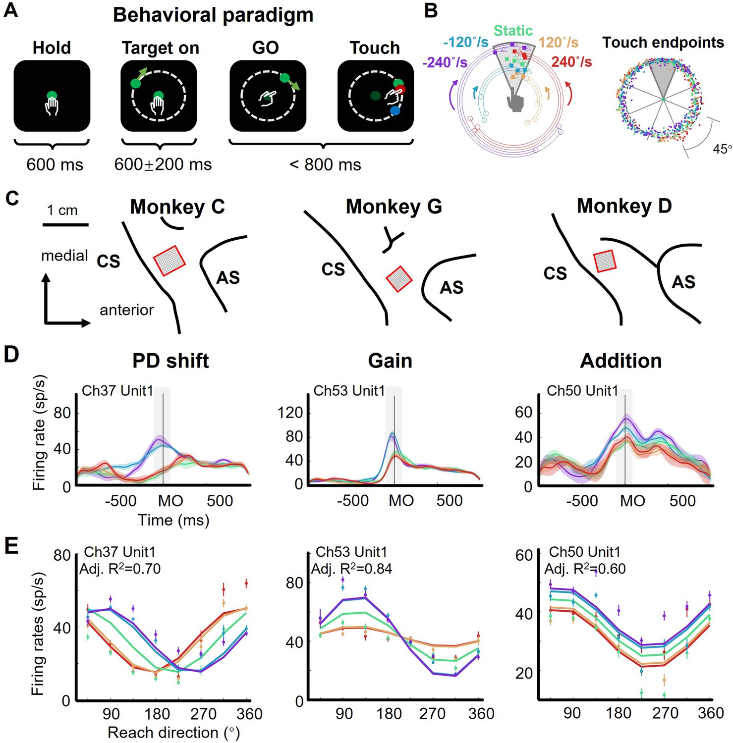
The flexible manual interception task and example neurons.
(A) Task diagram. In each trial, the monkey first holds the center dot for 600ms (Hold), then a target appears (Target on), after 400–800ms delay the center dot turns dark (GO), immediately the monkey moves its hand to reach to the target (Touch). The movement time (from GO to Touch) is required to be within 800ms, otherwise the trial will be aborted. The feedback dot, which is presented at the touched location of the screen, will be in red for success or in blue for failure. (B) Distribution of touch endpoints. Left panel shows fifteen reaching-up example trials in five target-motion conditions, three trials in each condition. The squares mark the touch endpoints, while the circles and triangles are the target onset and stop location. The five target-motion conditions (–240°/s, - 120°/s, 0°/s, 120°/s, and 240°/s) are indicated in five colors (purple, blue, green, yellow, and red). Target onset location is randomly distributed. Right panel shows the touch endpoints of all trials, each point represents a trial, colored according to target-motion conditions. The distribution was uniform around the circle (monkey C 772 trials, Rayleigh’s test, p=0.36). (C) Implanted locations of microelectrode array in the motor cortex of the three well-trained monkeys. Neural data were recorded from the cortical regions contralateral to the used hand. AS, arcuate sulcus; CS, central sulcus. (D) Three example neurons with PD shift, gain modulation, and offset addition. The peri-stimulus time histograms (PSTH) show the activity of example neurons when monkeys reached to upper areas in five target-motion conditions. The solid lines represent the trial-averaged firing rates, the colored shadow represents the standard error. The gray shadow indicates the time window between MO-100 ms and MO +100ms. (E) The directional tuning curves of the three example neurons with PD shift, gain, and addition modulation around movement onset (MO ±100ms, adjusted R2: 0.70, 0.84, and 0.60). Dots and bars denote the average and standard error of firing rates, colored according to target-motion conditions.
Figure 1—figure supplement 1
Flexible manual interception task and behavioral performance.
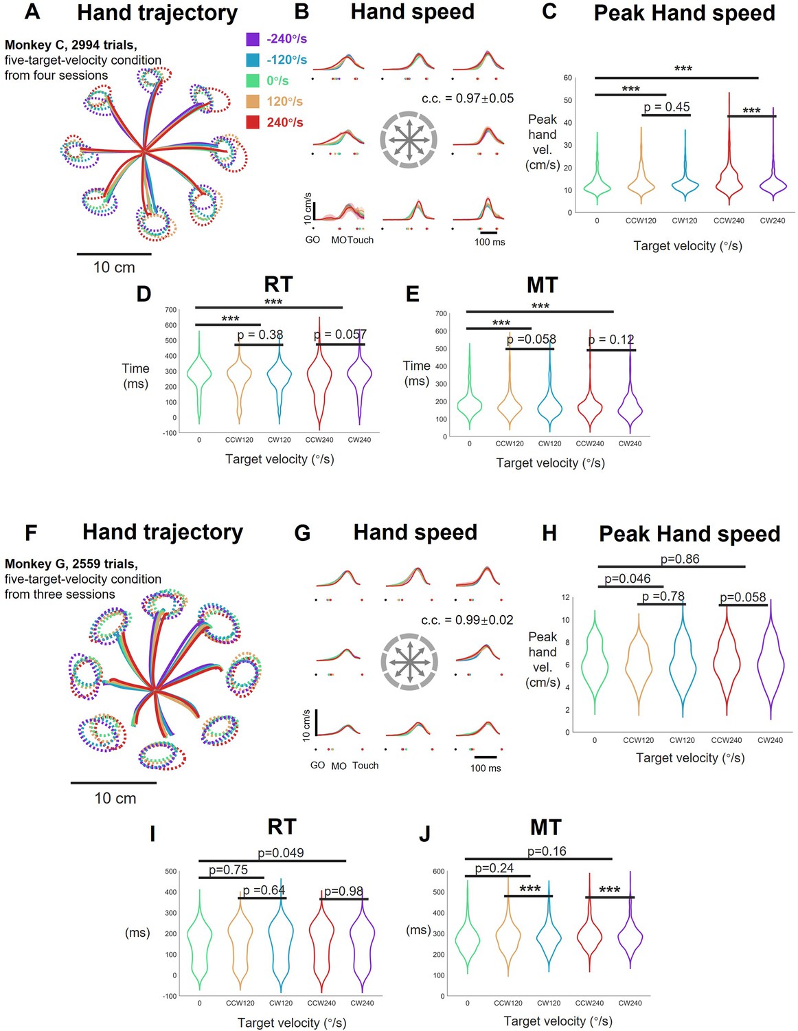
(A) The condition-averaged hand trajectory and touch endpoint distribution was averaged in five target-speed and eight reach-direction conditions (five colors) referred to target stopped location, including monkey C 2994 successful trials from four sessions. Hand trajectory was collected by optical camera (VICON Inc) with an infrared marker on the fingertip from GO to touching, and touch endpoint was collected by touchscreen. (B) The condition-averaged hand velocity was calculated from hand trajectory data (same in a), aligning to GO signal, with dots labelling GO (black), average movement onset (MO) and touch time (five color). Single-trial movement onset is defined as the moment of the first time rising to 5% of maximum hand velocity. The correlation coefficient of hand velocity profiles is 0.97±0.05, mean ± sd. of 40 conditions. (C) The trials distribution of peak hand velocity in five target-speed conditions (same in b). The peak hand velocity of static-speed condition were smaller than 120°/s and 240°/s conditions (ANOVA p-value of 0°/s vs. 120°/s, 120°/s vs. 240°/s were <10–6,<10–20). The hand velocity between CCW and CW had little difference (ANOVA p-value of CCW vs. CW was 0.45 within 120°/s and 10–4 within 240°/s). (D, E) The trials distribution in five target-speed conditions of reaction time and movement time (RT and MT, same sessions from monkey C). The temporal duration of static-speed condition were larger than 120°/s and 240°/s conditions (ANOVA p-value of 0°/s vs. 120°/s, 120°/s vs. 240°/s were <10–8 and<10–9 for RT, and <10–4 and<10–12 for MT). The duration between CCW and CW had little difference (ANOVA test). (F - G) The condition-averaged hand trajectory and velocity of monkey G 2559 successful trials from four sessions. (H - J) The trials distribution of peak hand velocity in five target-speed conditions, RT and MT (same sessions from monkey G, three starts mean ANOVA test p<0.01).
Figure 1—figure supplement 2
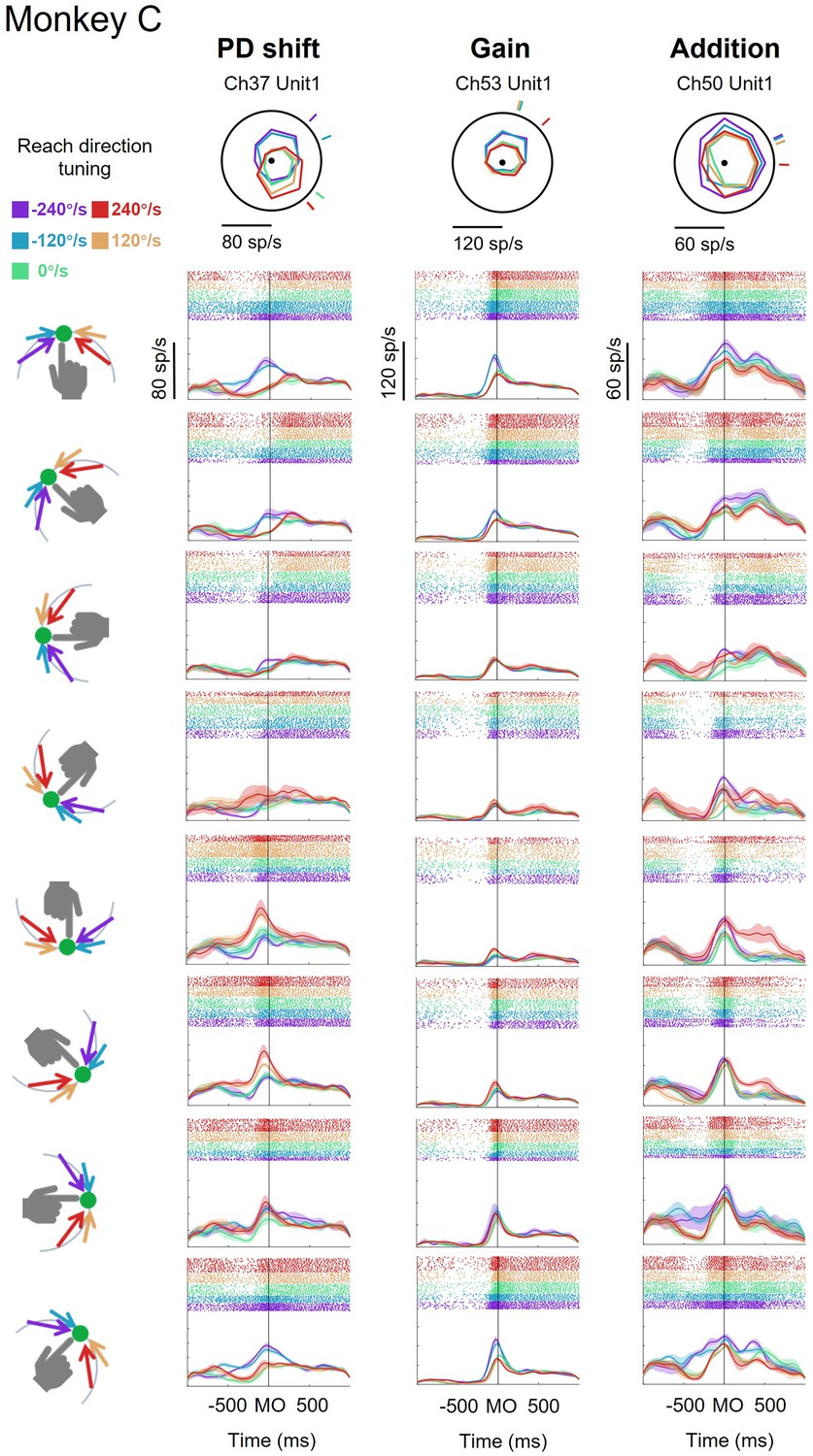
Three example neurons of monkey C.
Each column respectively showed threes example neurons with PD shift, gain modulation and offset modulation from monkey C (this figure), monkey G (Figure 1—figure supplement 3), and monkey D (Figure 1—figure supplement 4). The radar subplots in the first row showed the neuronal reach-direction tuning curves in five target-speed conditions (red, yellow, green, blue, and purple, for CCW 120, 240°/s, static, CCW 120, and 240°/s) at movement onset (MO ± 0.1 s), and short lines outside of the tuning curves labeled preferred directions. The next eight rows showed raters and peristimulus time histograms (PSTH) of example neuron activity to eight reaching areas (labeling in left, collecting the trials with touch endpoints in 45°) in five-target-speed conditions aligned to MO.
Figure 1—figure supplement 3
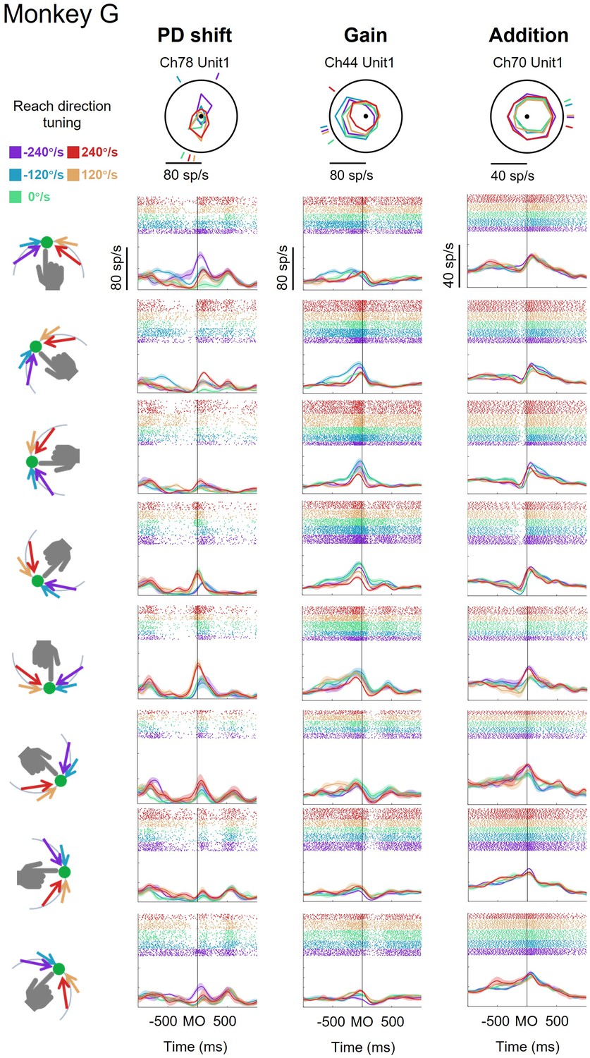
Three example neurons of monkey G.
Figure 1—figure supplement 4
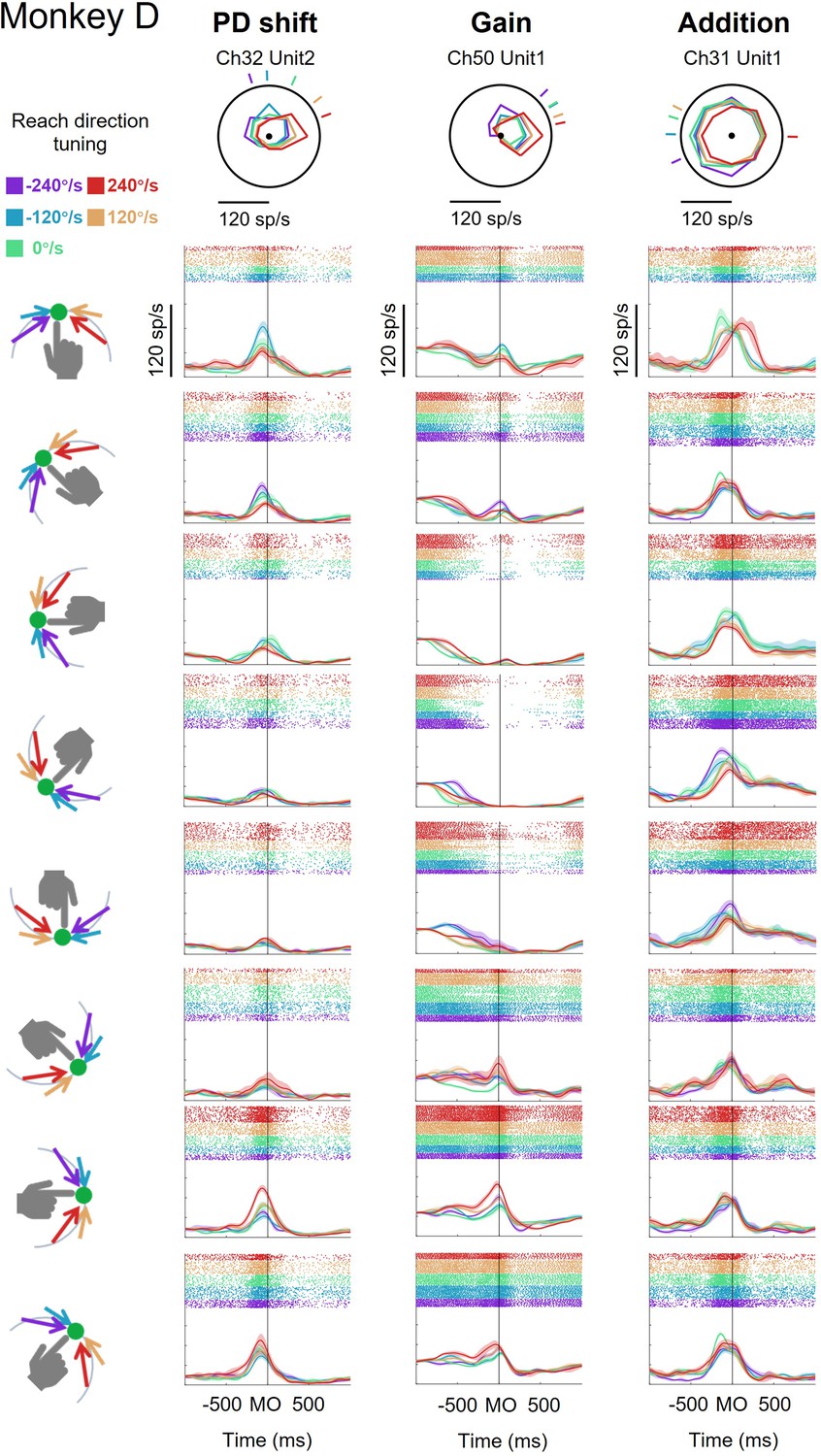
Three example neurons of monkey D.
Figure 1—figure supplement 5
Single-neuron fitting results.
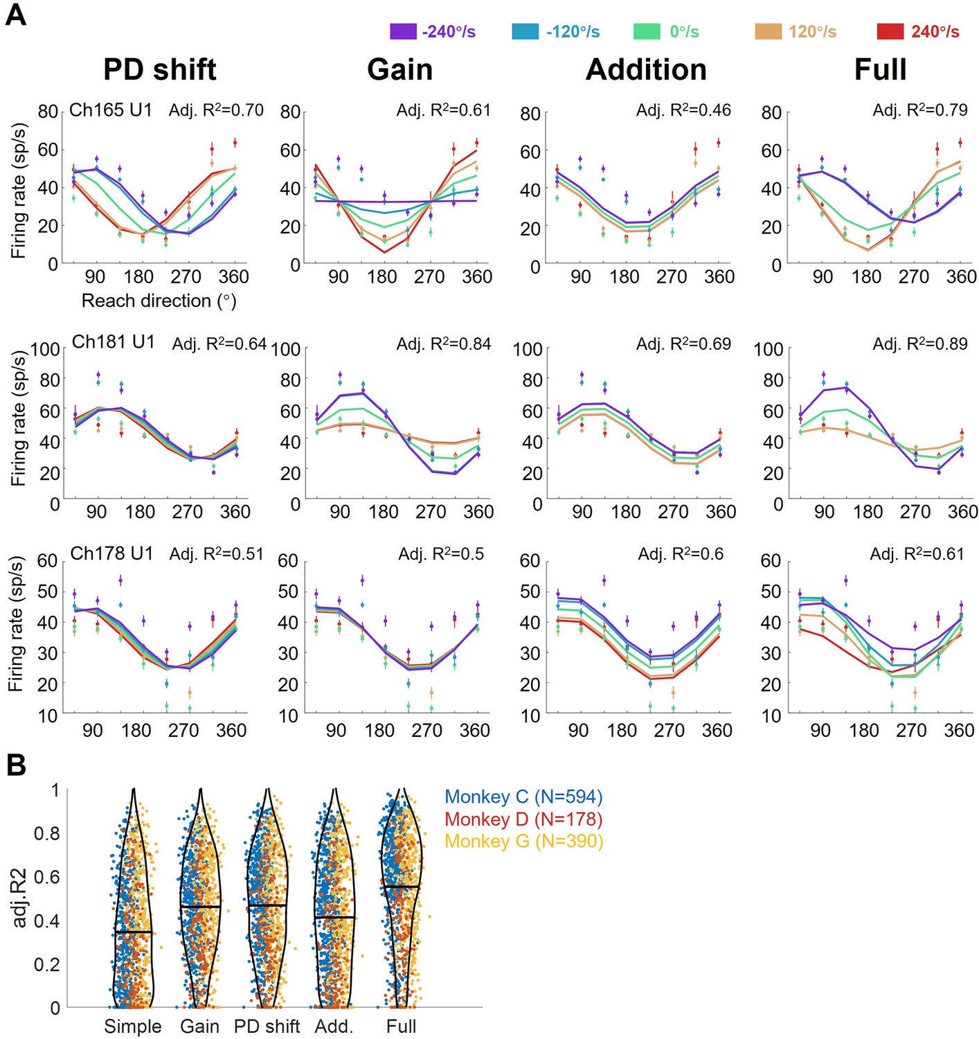
(A) The example condition-averaged neuronal activity with eight reach directions and five target speeds, fitted by PD shift, gain, offset, and full models. Dots and bars showed the condition average neuronal activity. Tuning curves were fitting results labeled with adjusted R-square at the top right. (B) The comparison of fitting goodness among five models (above four and simple model only fits reach direction with cosine function). Each dot shows the adjusted R-square of a single neuron (monkey C, N=594; monkey D, N=178; monkey G, N=390; in blue, red and yellow, respectively). Black bars are the mean of adjusted R-square (N=1162, simple model: 0.34±0.25, gain model: 0.46±0.22, PD shift model: 0.47±0.24, Addition model: 0.41±0.26, full model: 0.55±0.24, mean ± sd.). The adjusted R-squares of the full model are obviously larger than other models (Wilcoxon signed rank test, one-tailed, p<0.01).
Figure 2 with 4 supplements
Features of the encoding pattern at population level.
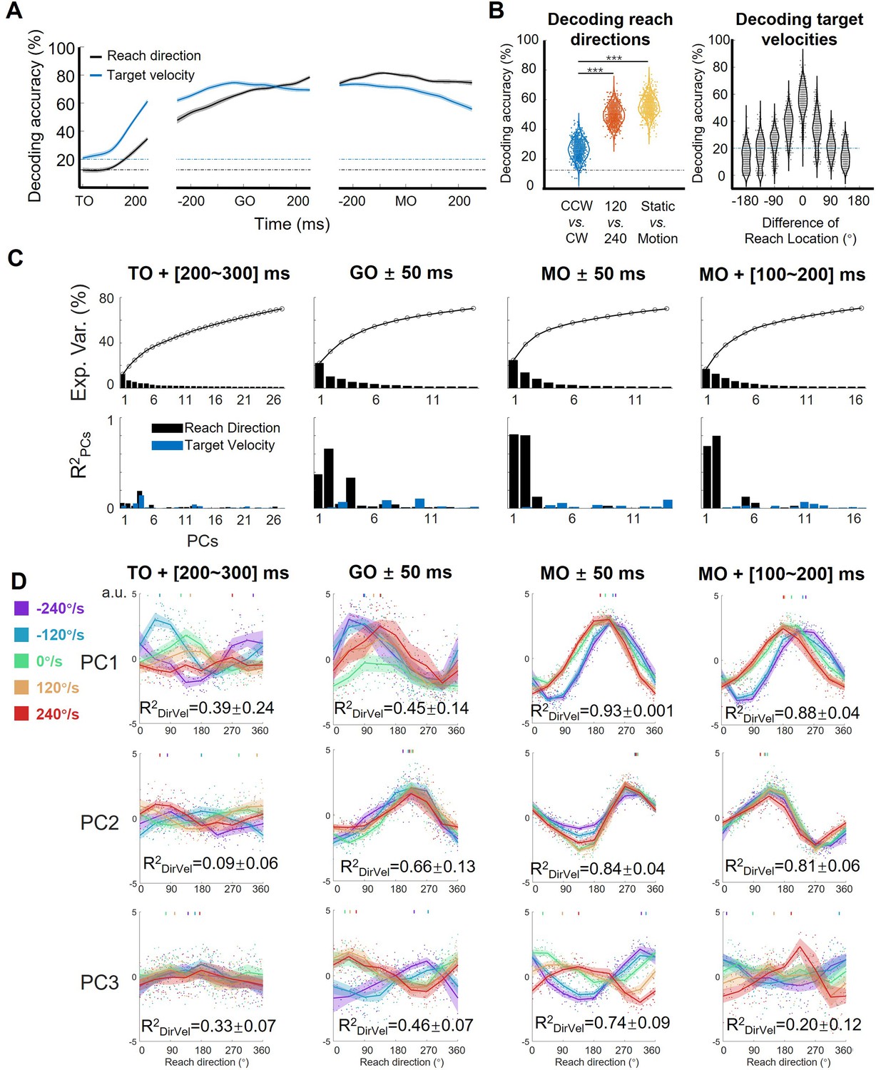
(A) The decoding accuracy (SVM with 10-fold cross-validation) of reach direction (black line) and target velocity (blue line) by population activity (monkey C, n=95, 772 trials), is aligned to target on (TO), GO, and movement onset (MO). The dash-dotted lines are chance level of decoding reach direction (black, one in eight) and target velocity (blue, one in five). The shaded area is the standard deviation of the decoding accuracy for 10 permutations. (B) The left panel shows the performance of reach-direction decoder (chance level: one in eight) transferred between different target-motion conditions. The SVM decoder was built on randomly selected 100 trials in training dataset and tested in another 100 trials from a dataset of different conditions (CCW vs. CW, 120 vs 240, static vs. motion). The distributions of decoding accuracy were from 1000 repetitions and compared with one tailed t-test (p<0.01, with three stars). The right panel shows the performance of target-velocity decoder (chance level: one in five) in different reach-direction conditions. The accuracy distribution was also obtained from 1000 repetitions. (C) The explained variance and representation of the principal components (PCs). The first row shows the explained variance of each PC (cumulatively over 70%). The second row shows the PCs’ fitting goodness (R2PCs) of reach direction and target velocity in four epochs. (D) Directional tuning curves of the PCs. Each row shows the directional tuning of one PC (the first three PCs in C) in four epochs. Each dot represents a trial, tuning curves are averaged in eight reach directions, and PDs of PCs are indicated by the short lines in the top of subplot by a weighted sum of response. The colors of the lines and dots mean the target-motion conditions, as the same as the legend on the left. The goodness of fitting reach direction (R2DirVel) for the single-trial PCs under single target-motion conditions is shown by mean ± sd. across conditions.
Figure 2—figure supplement 1
Decoding results of extended datasets.
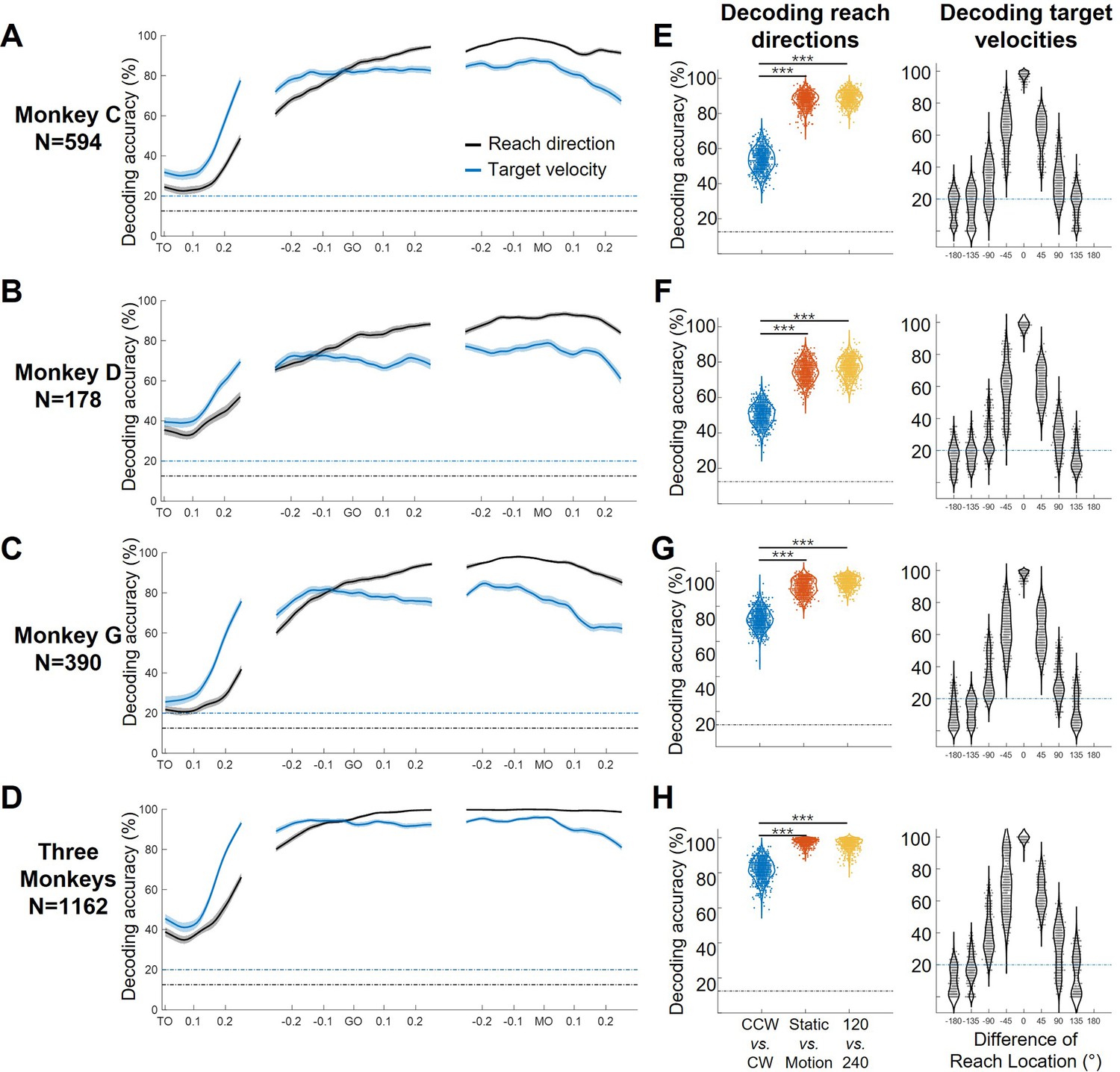
(A–D) The temporal decoding accuracy (SVM with 10-fold cross-validation) of reach direction (black line) and target speed (blue line) by pseudo-population activity (merged Monkey C, D, G, and all monkeys), is aligned to target on (TO), GO, and movement onset (MO). The dash-dotted lines are chance level of decoding reach direction (black, one in eight) and target speed (blue, one in five). The shaded area is the standard deviation of the decoding accuracy for 10 repetitions. (E–H) The left panel shows the performance of reach-direction decoder (one in eight) transferred between different target-motion conditions. The SVM decoder was built on randomly selected 100 trials in training dataset and tested in another 100 trials from a dataset of different conditions (CCW vs. CW, static vs. motion, 120 vs 240). The distributions of decoding accuracy were from 1000 repetitions and compared with one tailed t-test (p<0.01, with three stars). The right panel shows the performance of target-speed decoder (one in five) in different reach-direction conditions. In this case, reach direction is grouped by eight equal sectors (each 45°), and for each condition 60 trials were randomly selected for training and testing. The accuracy distribution was also obtained by 1000 repetitions.
Figure 2—figure supplement 2
Decoding results and neural states across epochs.
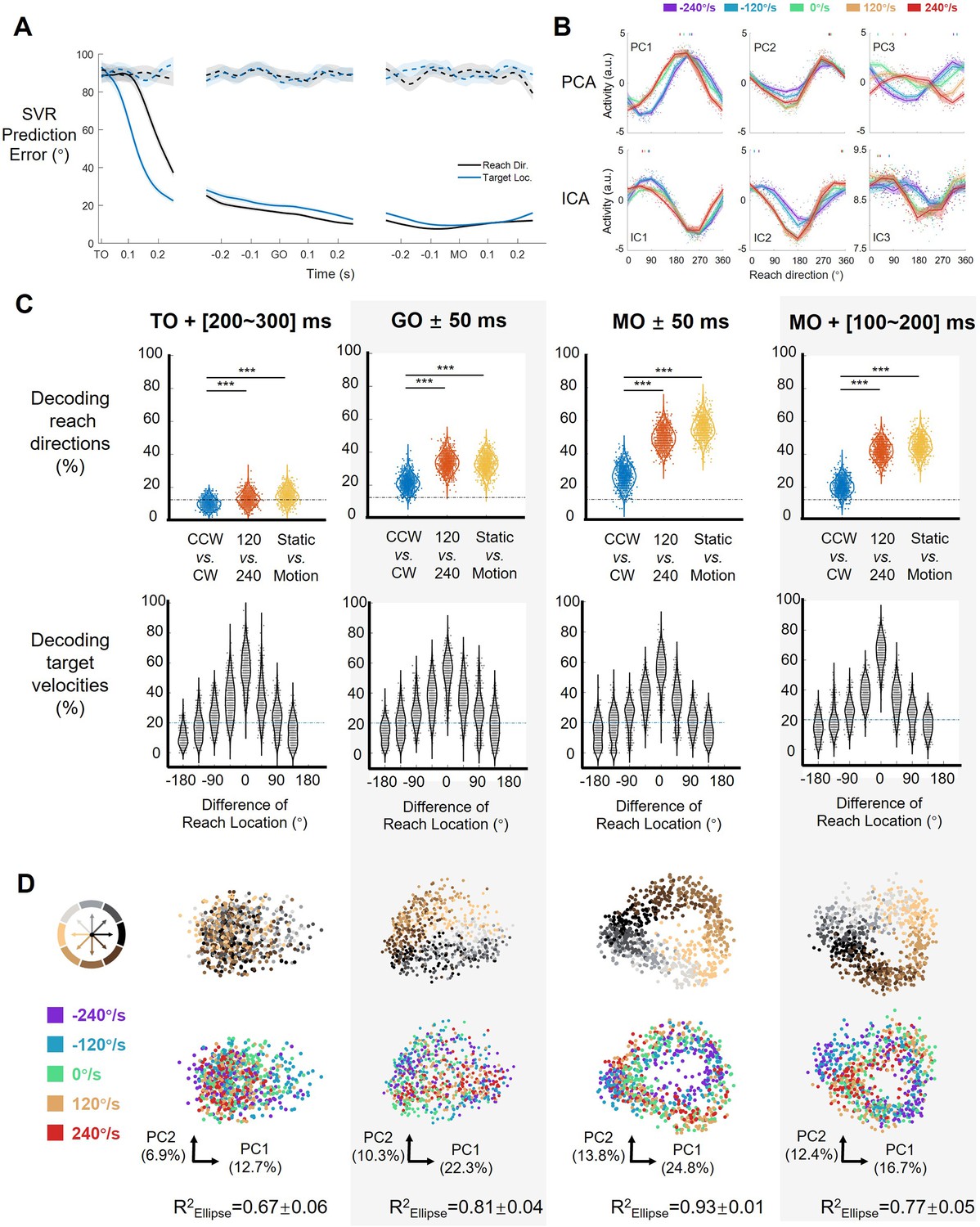
(A) The decoding accuracy (support vector regression, SVR with 10-fold cross-validation) of reach direction (black line) and simultaneous target direction (blue line) on population activity (monkey C, n=95, 772 trials), is aligned to target on (TO), GO, and movement onset (MO). The dotted lines represent the chance level of decoding reach direction (black) and target direction (blue) using data with shuffled trial labels. The line and shaded area indicate the mean and standard error of the decoding accuracy for trials. (B) Results of unsupervised dimensionality reduction on the example dataset. Each subplot shows the directional tuning of one component at movement onset (PCAs are the same with Figure 2D). Each dot represents a trial, and tuning curves are averaged by eight reach directions and colored by target-motion conditions. The short lines at the top of the subplot show corresponding PDs by a weighted sum of response. (C) Decoders generalize between conditions in several epochs. The first row shows the performance of reach-direction decoder (chance level: one in eight) transferred between different target-motion conditions. The SVM decoder was built on randomly selected 100 trials in training dataset and tested in another 100 trials from a dataset of different conditions (CCW vs. CW, 120 vs 240, static vs. motion). The distributions of decoding accuracy were from 1000 repetitions and compared with one tailed t-test (p<0.01, with three stars). The second row shows the performance of target-speed decoder (chance level: one in five) in different reach-direction conditions. In this case, reach directions are grouped by eight equal sectors (each 45°), and for each condition 60 trials were randomly selected for training and another 60 (?) for testing. The accuracy distribution was also obtained from 1000 repetitions. (D) The neural states across epochs. In this plane spanned by the first two PCs, the dots represent the single-trial neural states in color corresponding to reach directions (first row) or target speed (second row). The explained variance is marked on the corresponding axes. The goodness of fitting ellipses (R2Ellipse) for the state dots is shown as mean ± sd across single target-motion conditions.
Figure 2—figure supplement 3
dPCA and subspace projection.
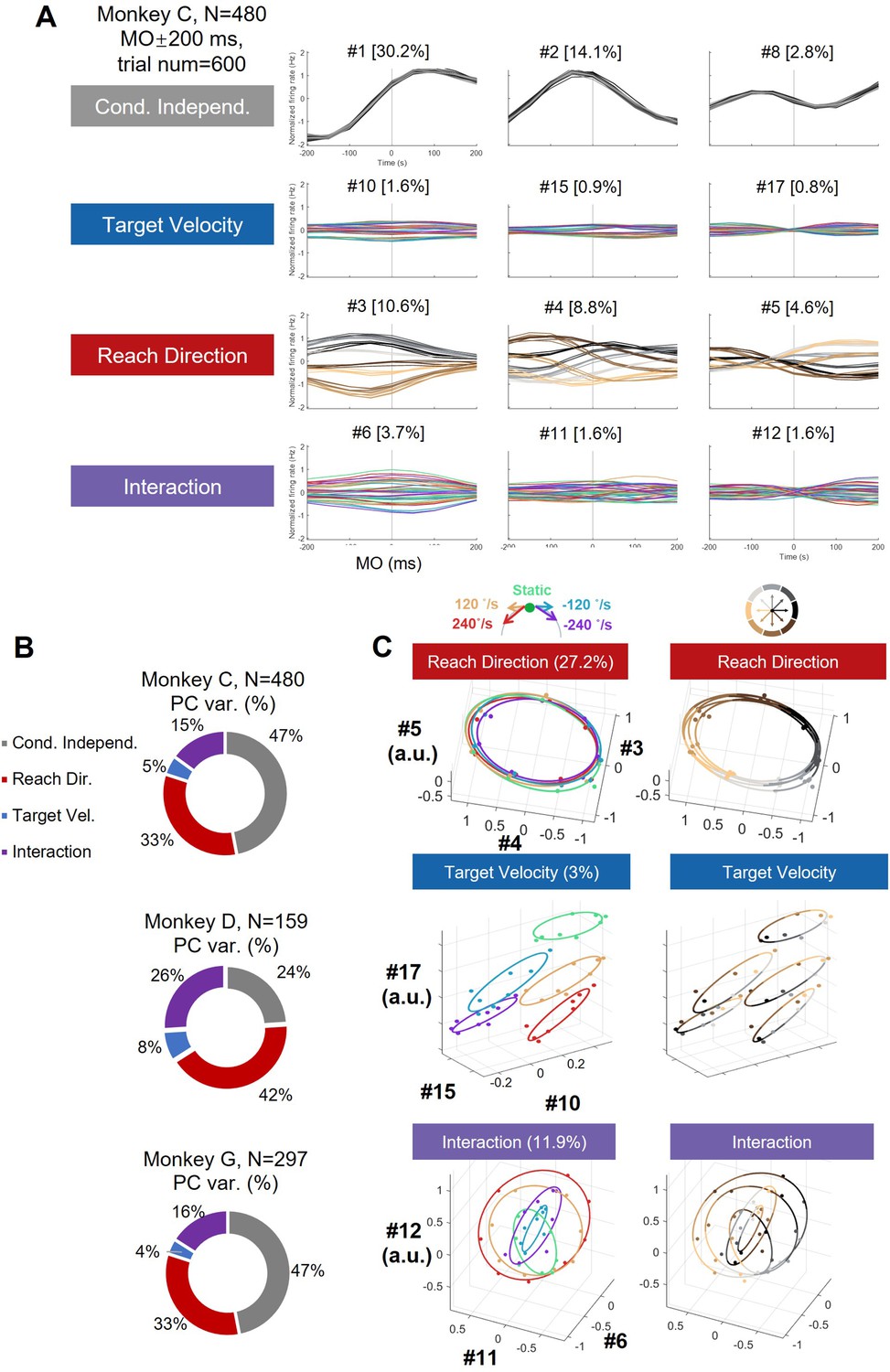
(A) Neural data were merged by target-speed modulated units (N=480, K=600 trials, T=8, bin = 50 ms, from 6 sessions of monkey C) and were averaged into 40 conditions (NKT = [480,40,8]) to do dPCA (Kobak et al., 2016). The condition independent components are colored as reach direction, and the interaction components are colored as target-motion conditions. (B) Summary dPCA components variance for three monkeys merged datasets. (C) Neural states in ‘reach-direction subspace’, ‘target-velocity subspace’, and ‘interception subspace’. We used dPCA components with different features to construct three subspaces (same data in A, reach-direction space #3, #4, #5; target-velocity space #10, #15, #17; interaction space #6, #11, #12), and we projected trial-averaged data into these orthogonal subspaces using different colormaps. This approach allowed us to obtain a ‘potent subspace’ coding reach direction and a ‘null space’ for target velocity. The results showed that the reach-direction subspace effectively represented the reach direction. However, while the target-velocity subspace encoded the target velocity information, it still contained reach-direction clusters within each target-velocity condition, corroborating the results of the addition model in the main text (Figure 4). The interaction subspace revealed that multiple reach-direction rings were nested within each other, similar to the findings from the gain model (Figures 3 and 4). The interaction subspace also captured more variance than target-velocity subspace, consistent with our PCA results, suggesting the target-velocity modulation primarily coexists with reach-direction coding. Furthermore, we explored alternative methods to verify whether orthogonal subspaces could effectively separate the reach direction and target velocity. We could easily identify the reach-direction subspace, but its orthogonal subspace was relatively large, and the target-velocity information exhibited only small variance, making it difficult to isolate a subspace that purely encodes target velocity.
Figure 2—figure supplement 4
Neural trajectory during preparatory and peri-movement periods.
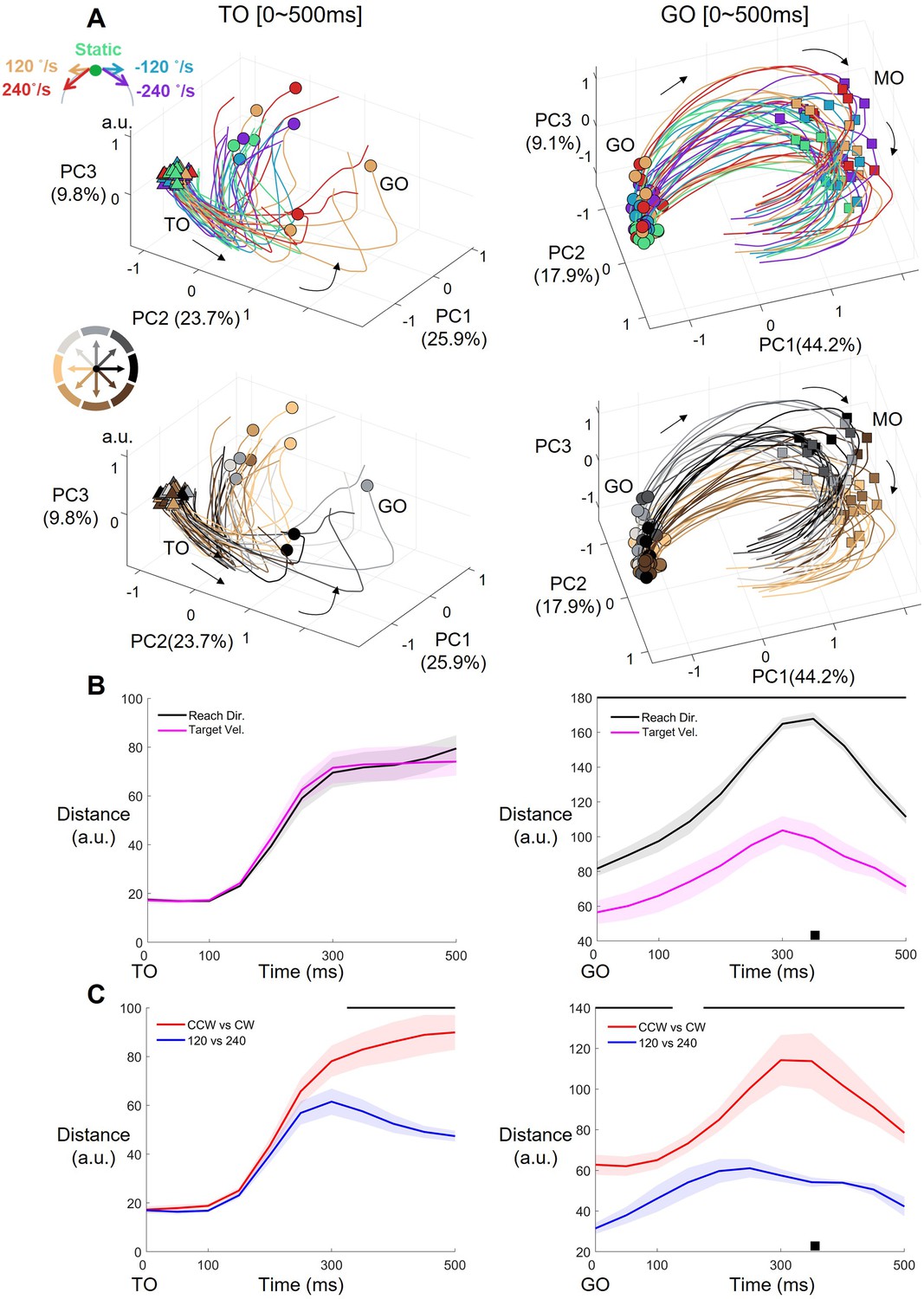
(A) The first three dimension of the condition-averaged neural trajectory (Monkey C, n=95, 40 conditions) in two periods. The neural data was N*KT (N for 95 neurons, K for 40 conditions combined with T=10 bins, bin length 50 ms, 40 conditions contain a combination of five target speeds and eight reach directions), and reduced neural dimension N to explain KT with PCA (explained variance of PC labeling in parentheses). Left column is delay period (TO to TO +500 ms, TO means target onset), with triangles and circles labeling condition-averaged TO and GO. Right column is peri-movement period (GO to GO +500 ms), with circles and squares labeling GO and movement onset (MO). The same neural trajectory is plotted in two colormaps with target-motion conditions (up row) and reach directions (down row). Black arrows mark the direction of temporal evolution. (B) The mean neural trajectory Euclidian distance of target-motion and reach-direction conditions, aligned to TO (left) and GO (right), respectively, with selected 8 PCs and 14 PCs respectively covering 90% of delay period and movement period data variance. The black bar above the subplot labels the obvious difference temporal bin between two distances (Kruskal-Wallis test, p<0.05). The shadow means the standard error. The black square is the condition-averaged MO. (C) The mean neural trajectory Euclidian distance with same data in B, comparing CCW vs. CW and 120 vs 240 conditions.
Figure 3 with 2 supplements
The orbital neural geometry in latent dynamics.
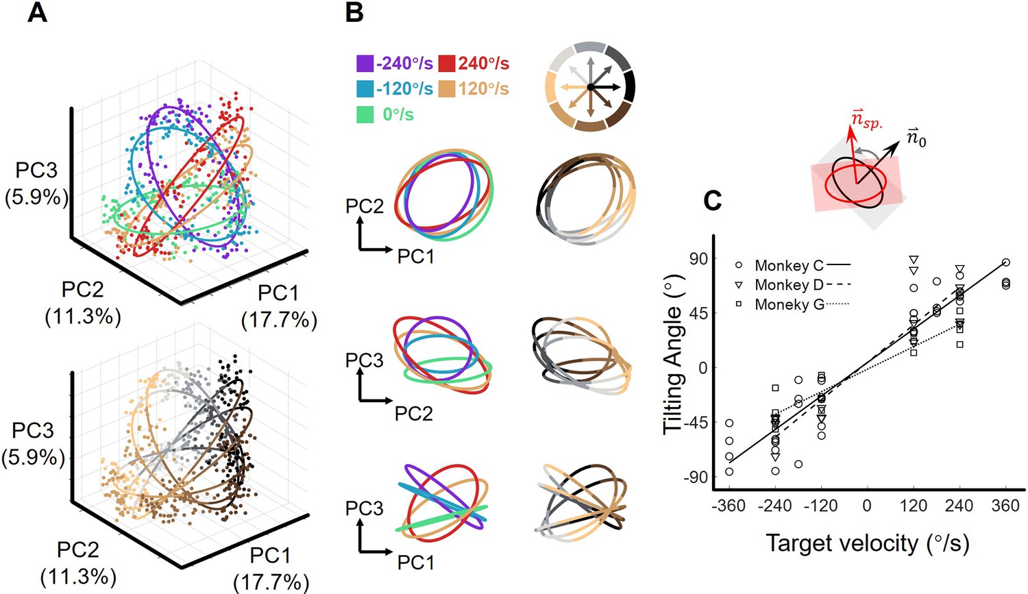
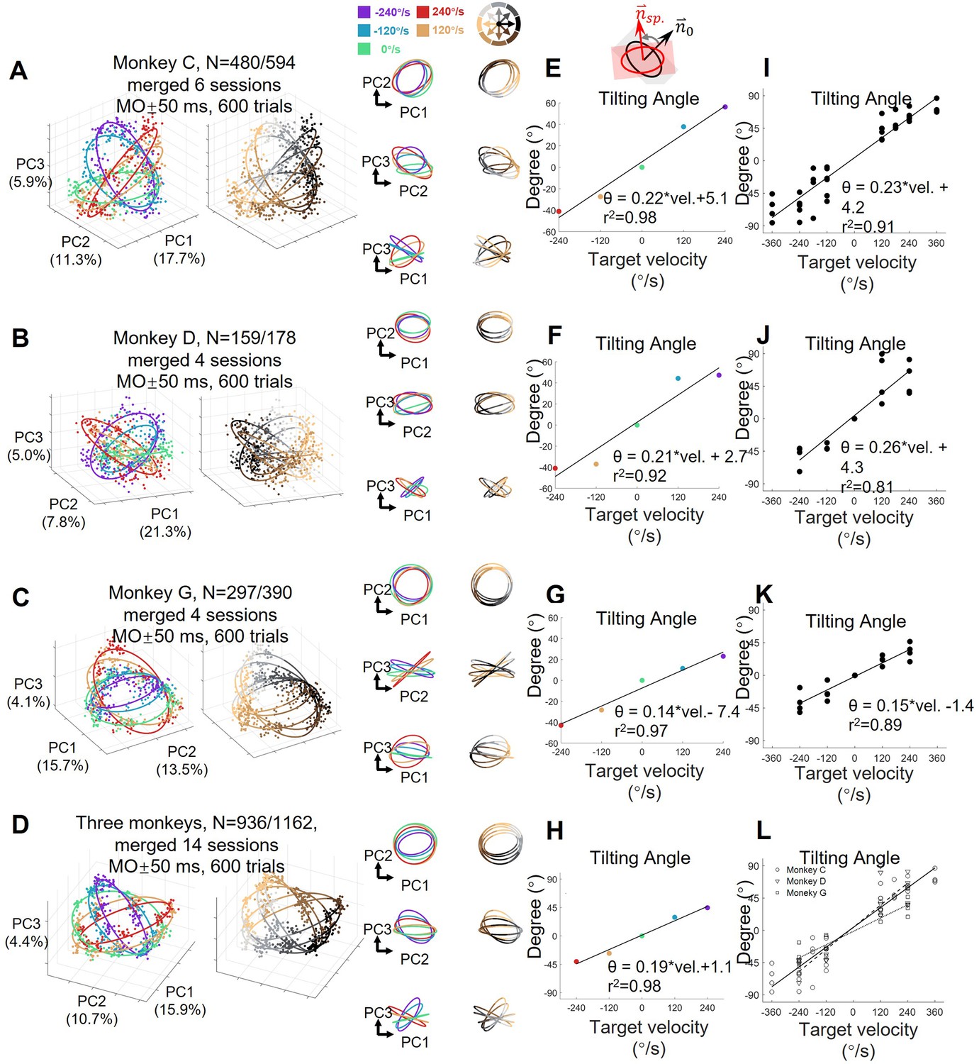
(A) Three-dimensional neural state of M1 population activity obtained by PCA. Each point represents a single trial. The upper subplot is colored according to five target-motion conditions, while the bottom is in colors corresponding to eight reach directions. The explained variances of the first three PCs were 17.7%, 11.3%, and 5.9%. Neural data were from monkey C (N=480, merged six sessions), for each of the total 40 conditions, 15 trials were randomly sampled. (B) Fitted ellipses of neural states. The ellipses fitted in (A) are projected onto three two-dimensional subspaces, colored by target velocities (left column) or reach directions (right column). (C) The relation between the tiling angle and target velocity. The tilting angle is calculated between ellipses of the moving-target conditions and the static-target condition (0 °/s) in the range from –90° to 90°, CCW is defined as positive. Circles, squares, and triangles correspond to monkeys C (7 sessions), G (4 sessions), and D (4 sessions), respectively. The lines indicate the linear fitting between the tilting angle (θ) and target velocity (vel.), with solid line for monkey C (θ=0.23*vel.+4.2, R2=0.91), dashed line for monkey D (θ=0.26*vel.+4.3, R2=0.81), and dotted line for monkey G (θ=0.15*vel.-1.4, R2=0.89).
Figure 3—figure supplement 1
Neural state of target-motion modulated M1 neurons from three monkeys.
The neural state of movement onset (MO ± 50ms) from three-monkey selected neurons. Neural data was collected with target-speed modulated units (N) and random 15 trials in 40 conditions (K=600 trials) from each monkey several sessions (A–C) and all monkeys’ sessions (D). Merged neural data was to do PCA to get neural state. Each point represented the neural state of single trial projected in static condition subspace. Ellipses were fitted by neural states in five target-speed conditions. (E–H) The relative titling angle of ellipses from static condition (merged datasets), had a linear relationship with target speed. Five color dots were tilting angles of five-target-speed condition. (I–L) We calculated the titling angle for separative sessions, and got the consistent linear relationship between tilting angle and target speed. The titling angle of three monkeys also showed in Figure 3.
Figure 3—figure supplement 2
Target-motion modulation on hand-speed-filtered trials.
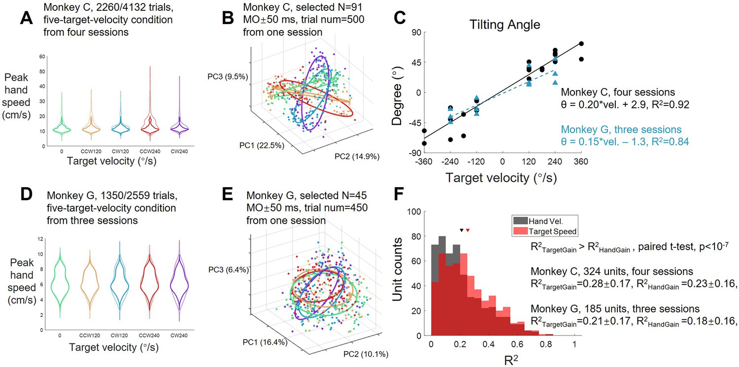
(A) The peak hand velocity distribution with selected trials. We used 10~90% of peak hand velocity in static-speed condition as threshold to select trials. Solid lines are remaining-trial distribution (monkey C 2260/4132 trials) and dash lines are raw distribution in Figure 1—figure supplement 1. After filtering, there is no difference between five-speed conditions (ANOVA p-value of 0°/s vs. 120°/s, 0°/s vs. 240°/s, and 120°/s vs. 240°/s were 0.56, 0.14, and 0.26). (B) Adjusted neural state with filtered trials. We performed PCA to neural data of one example session with filter trials (random chose 100 trials for each target-speed condition by a filter of 10~90% of peak hand velocity in static-speed condition, K=500 trials) and selected units (target-speed modulated neuron, N=91), to get neural state. We repeated in each sessions of two monkeys, then neural states of target-speed conditions were fitted ellipses and calculated the tilting angles of ellipses. (C) Tilting angle between ellipses of adjusted neural state. The titling angles were highly correlated with target speed (black circles and blue triangle are four sessions of monkey C, and three sessions of monkey G). (D) The filtered hand-velocity distribution compared with raw distribution (dashed line, Figure 1—figure supplement 1H). (E) Adjusted neural state of one example session from monkey G. (F) The R2 distribution of single-unit gain model. The gain of target speed performed better than hand velocity, with fr = c0+a*(y+c1)*cos(x-b)+c2*y, fr was mean firing rate of MO ± 50ms, x for reach direction, y for target speed or hand velocity. The triangles labeled the mean R2 of two models.
Figure 4
The shape of neural dynamics relies on neuronal mixed selectivity.
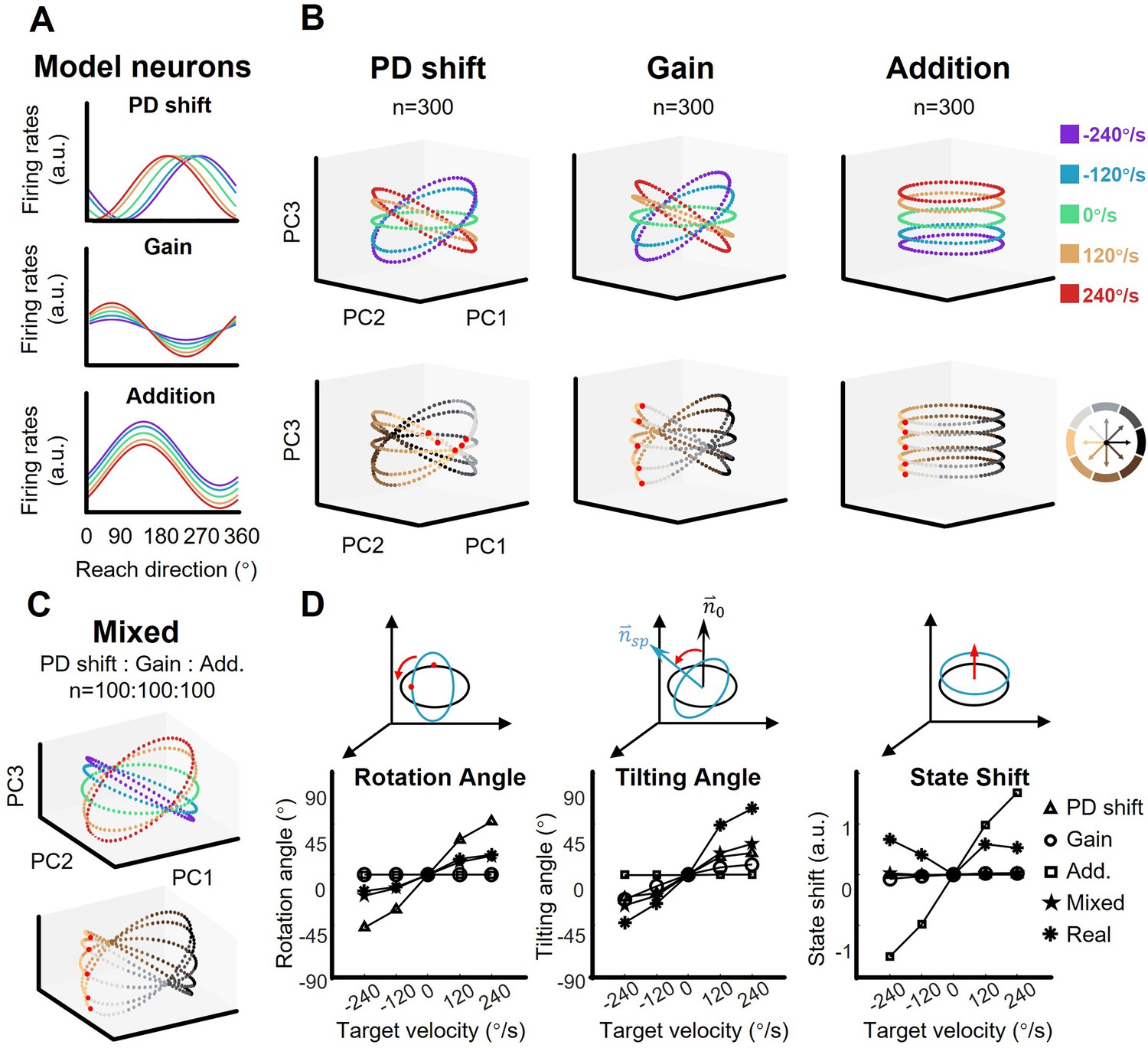
(A) The tuning curves of three ideal neurons in five target-motion conditions. From up to down, they are PD shift, gain modulation, and addition. (B) The simulated neural states from three groups of ideal neurons, colored according to target-motion conditions (first row) and reach directions (second row). For each simulation, the neural states were obtained from 300 model neurons by PCA. The neural state in 180° reach direction is marked with a red dot. The first two principal components (PCs) can explain more than 95% of the variance in the data (the explained variance of the first three PCs, Gain: 49.5%, 46.6%, and 2.0%; PD shift: 50.1%, 47.1%, and 1.6%; Addition:50.8%, 47.9%, and 1.4%). (C) The neural states of a mixed group of 100*3 model neurons, as in (B). The explained variance of the first three PCs were 48.4%, 44.2%, and 3.1%. (D) Quantification of the difference between neural-state ellipses in four simulated groups and a real dataset (monkey C, n=95). Rotational angle is the angular differences in the first two neural state. Tilting angle is the relative angle of the normal vector of ellipses. State shift is the root of mean squared distance between two ellipses.
Figure 5 with 1 supplement
The neural geometry in RNNs.
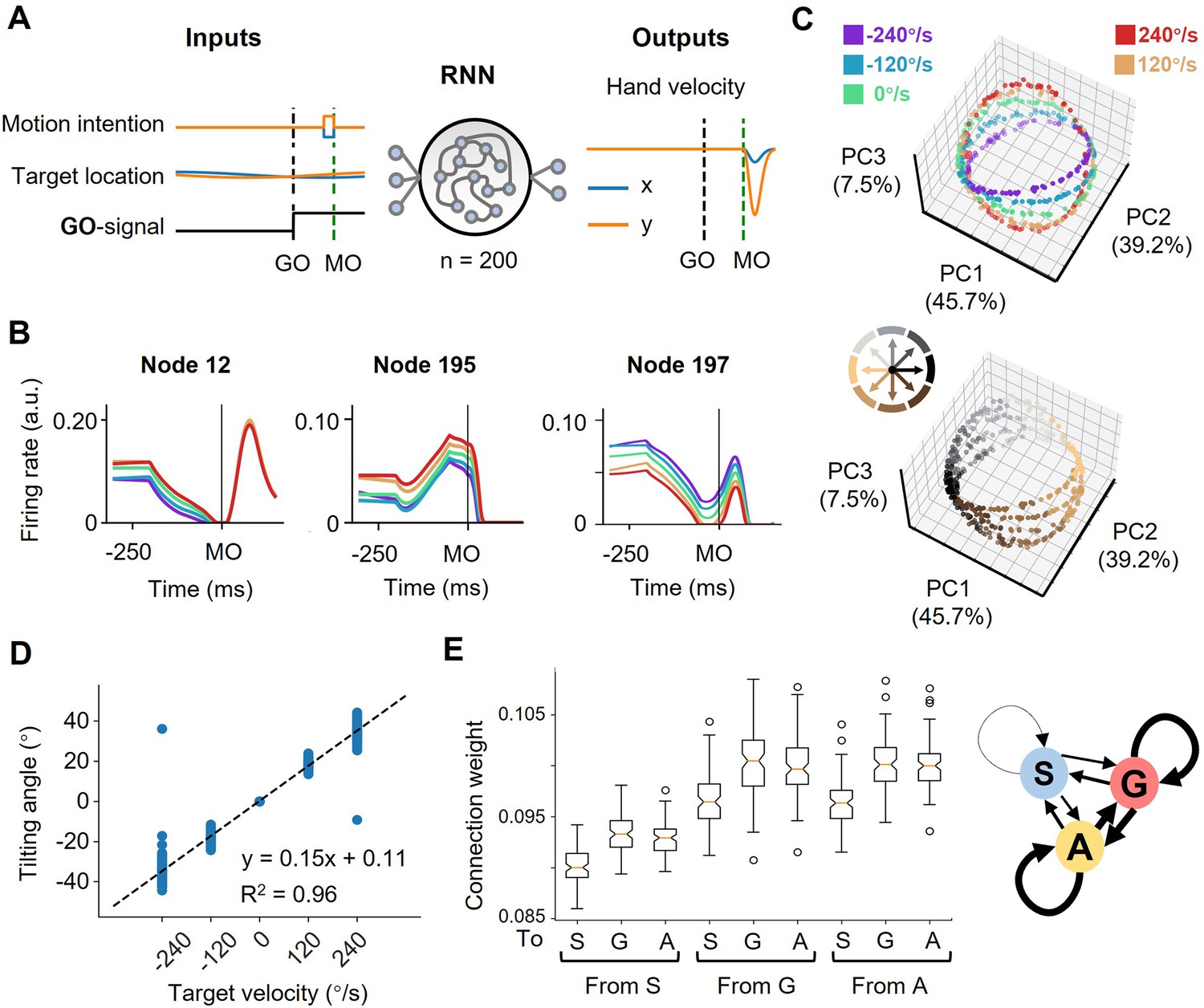
(A) Network architecture. The network inputs consist of motor intention, target location, and GO signal. The motor intention is the two-dimensional Cartesian coordinate of the interception location, and exists fixed during MO-50ms to MO; the target location is the two-dimensional Cartesian coordinate of the moving target, and appears time-varying during the whole trial; the GO-signal is a step function, jumping from 0 to 1 at GO. The RNN with 200 hidden units is expected to output hand velocity in two-dimensional Cartesian coordinates for accurate interception. (B) Three example nodes with PD-shift modulation, gain modulation, and additive modulation. Similar to Figure 1D. (C) Three-dimensional neural state of node activity obtained by PCA, colored according to target-motion conditions (top) and reach-direction conditions (Bottom). Similar to Figure 3A. (D) The tilting angle of ellipses. Similar to Figure 3D. The fitted line is θ=0.15*vel.+0.11, R2=0.96, across five target velocities. (E) The connectivity between different types of modulations. On the left is a boxplot representing the averaged absolute connection weight, across 100 models. S for PD-shift nodes, G for gain nodes, and A for additive nodes. On the right is a diagram of the connectivity, with linewidth representing the relative connection strength.
Figure 5—figure supplement 1
Decoding results and weight distributions of RNNs.
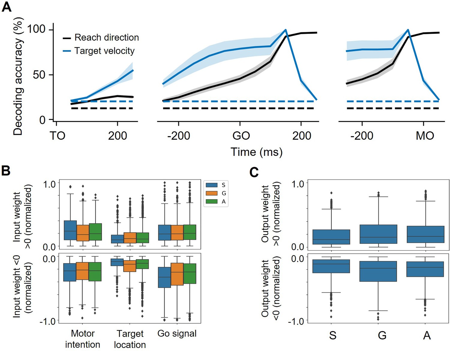
(A) The decoding accuracy (SVM with 10-fold cross-validation) of reach direction (black line) and target speed (blue line) across 100 network models, is aligned to TO, GO, MO. The dash-dotted lines are chance level of decoding reach direction (black, one in eight) and target speed (blue, one in five). While the lines are the mean of the mean decoding accuracy across models, the shaded area is the standard deviation of the mean decoding accuracy across models. (B) The input weights. The weights from motor intention-x and motor intention-y were averaged as motor intention, so as target location-x and target location-y to target location. To get a relative tendency, we selected the only modulated nodes and normalized the weight by dividing the maximum (the max absolute weight from motor intention, target location, and GO-signal, respectively), for each model. For motor intention (weight >0), S>G = A; for target location, S<G = A (weight >0), S<A < G (weight <0); for GO-signal (weight <0), S>G = A. ‘=’ here defines no significance while ‘<’ means p<0.01. (C) The output weights. The outputs to x and y were averaged. Similar with B, we selected the only modulated nodes and normalized the weight by dividing the max absolute output weights, for each model. No matter whether weight >0, S<G = A (p<0.001).
Tables
Table 1
Ratio of mixed selectivity neurons around movement onset.
| Units across sessions | Gain (G) | PD shift (S) | Addition (A) | None |
|---|---|---|---|---|
| Monkey C, 7 sessions, N=84.9 ± 15.9 | 46.9 ± 15.9% | 79.0 ± 8.9% | 61.9 ± 14.5% | 6.5 ± 6.2% |
| Monkey G, 4 sessions, N=97.5 ± 17.7 | 29.3 ± 4.9% | 51.6 ± 29.1% | 25.9 ± 8.3% | 25.5 ± 15.8% |
| Monkey D, 4 sessions, N=44.5 ± 7.5, | 45.6 ± 13.8% | 74.4 ± 8.8% | 49.1 ± 9.1% | 10.8 ± 5.4% |
| RNN, N=200, 100 models | 46.5 ± 4.6% | 40.7 ± 4.2% | 57.9 ± 8.9% | 14.2 ± 4.2% |
-
Single neurons were classified by modulation patterns (more details in Materials and methods). The first column shows the subject, the number of recording sessions, and the number of isolated units (mean ± sd.). Other columns show the ratio of units with any target-velocity modulations in all active units. ‘None’ means the units were not specifically tuned by either reach direction nor target velocity.
Additional files
-
Supplementary file 1
Neural datasets.
- https://cdn.elifesciences.org/articles/100064/elife-100064-supp1-v1.docx
-
Supplementary file 2
Neural dynamics similarity.
- https://cdn.elifesciences.org/articles/100064/elife-100064-supp2-v1.docx
-
Supplementary file 3
RNN perturbation results.
- https://cdn.elifesciences.org/articles/100064/elife-100064-supp3-v1.docx
-
Supplementary file 4
Alternative models.
- https://cdn.elifesciences.org/articles/100064/elife-100064-supp4-v1.docx
-
MDAR checklist
- https://cdn.elifesciences.org/articles/100064/elife-100064-mdarchecklist1-v1.docx
Download links
A two-part list of links to download the article, or parts of the article, in various formats.
Downloads (link to download the article as PDF)
Open citations (links to open the citations from this article in various online reference manager services)
Cite this article (links to download the citations from this article in formats compatible with various reference manager tools)
Neural geometry from mixed sensorimotor selectivity for predictive sensorimotor control
eLife 13:RP100064.
https://doi.org/10.7554/eLife.100064.3


