The emergence of visual category representations in infants’ brains
- Department of Psychology, Stanford University, United States
- Wu Tsai Neurosciences Institute, Stanford University, United States
- Institute of Science and Technology for Brain-Inspired Intelligence, Fudan University, China
- Neurosciences Program, Stanford University, United States
Figures
Figure 1
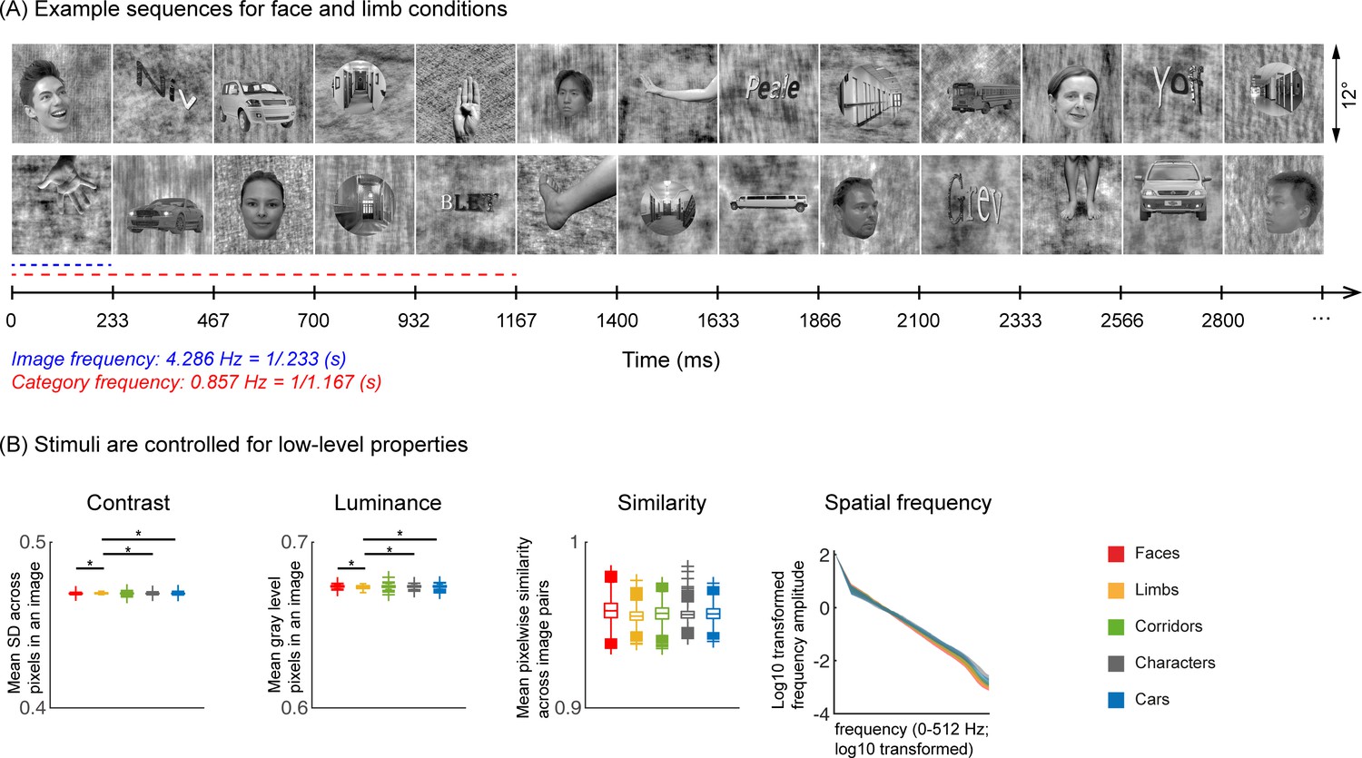
Experimental design and stimuli analysis.
(A) Example segments of presentation sequences in which faces (top panel) and limbs (bottom panel) were the target category. Images spanning 12° containing gray-level images of items from different categories on a phase-scrambled background appeared for 233 ms (frequency: 4.286 Hz). A different exemplar from a single category appeared every fifth image (frequency: 0.857 Hz). Between the target category images, randomly drawn images from the other four categories were presented. Sequences consisted of 20% images from each of the five categories and no images were repeated. Each category condition lasted for 14 s and contained 12 such cycles. Participants viewed in random order 5 category conditions: faces, limbs, corridors, characters, and cars forming a 70 s presentation sequence. (B) Images were controlled for several low-level properties using the SHINE toolbox as explained in Stigliani et al., 2015. Metrics are colored by category (see legend). Contrast: mean standard deviation of gray-level values in each image, averaged across 144 images of a category. Luminance: mean gray-level of each image, averaged across 144 images of a category. Similarity: mean pixel wise similarity between all pairs of images in a category. For all three metrics, boxplots indicate median, 25%, 75% percentiles, range, and outliers. Significant differences between categories are indicated by asterisks, for contrast and luminance (nonparametric permutation t-test p<0.05, Bonferroni corrected); for image similarity, all categories are significantly different than others (nonparametric permutation testing, p<0.05, Bonferroni corrected, except for corridors vs. cars, p=0.24). Spatial frequency: Solid lines: distribution of spectral amplitude in each frequency averaged across 144 images in each category. Shaded area: standard deviation. Spatial frequency distributions are similar across categories.
Figure 2
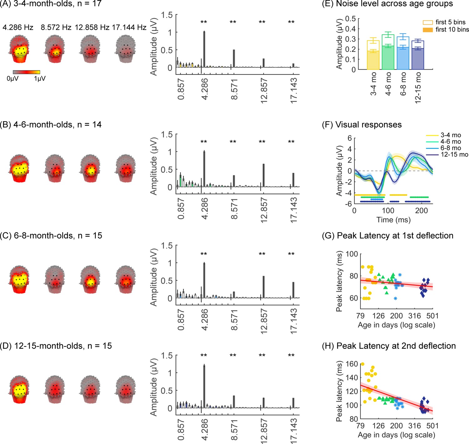
Strong visual responses over occipital cortex at the image-update frequency and its harmonics in all age groups.
Each panel shows mean responses across infants in an age group. (A) 3- to 4-month-olds, n=17; (B) 4- to 6-month-olds, n=14; (C) 6- to 8-month-olds, n=15; (D) 12- to 15-month-olds, n=15. Left panels in each row: spatial distribution of the visual response at the image-update frequency and its first three harmonics. Middle panels in each row: mean Fourier amplitude spectrum across nine occipital electrodes of the occipital region of interest (ROI) showing high activity at harmonics of the image-update frequency marked out by thicker lines. Data are first averaged in each participant and each condition and then across participants. Error bars: standard error of the mean across participants. Asterisks: response amplitudes significantly larger than zero, p<0.01, false discovery rate (FDR) corrected. Colored bars: amplitude of response at category frequency and its harmonics. White bars: amplitude of response at noise frequencies. (E) Noise amplitudes in the frequency range up to 8.571 Hz (except for the visual response frequencies and visual category response frequencies) from the amplitude spectra in (A) for each age group (white bars on the spectra). Error bars: standard error of the mean across participants. (F) Mean image-update response over occipital electrodes for each age group. Waveforms are cycle averages over the period of the individual image presentation time (233 ms). Lines: mean response. Shaded areas: standard error of the mean across participants of each group. Horizontal lines colored by age group: significant responses vs. zero (p<0.05 with a cluster-based analysis, see Methods). (G) Peak latency for the first peak in the 60–90 ms interval after stimulus onset. Each dot is a participant; dots are colored by age group. Line: linear mixed model (LMM) estimate of peak latency as a function of log10(age). Shaded area: 95% confidence interval (CI). (H) Same as (G) but for the second peak in the 90–160 ms interval for 3- to 4-month-olds, and 90–110 ms for older infants.
Figure 3
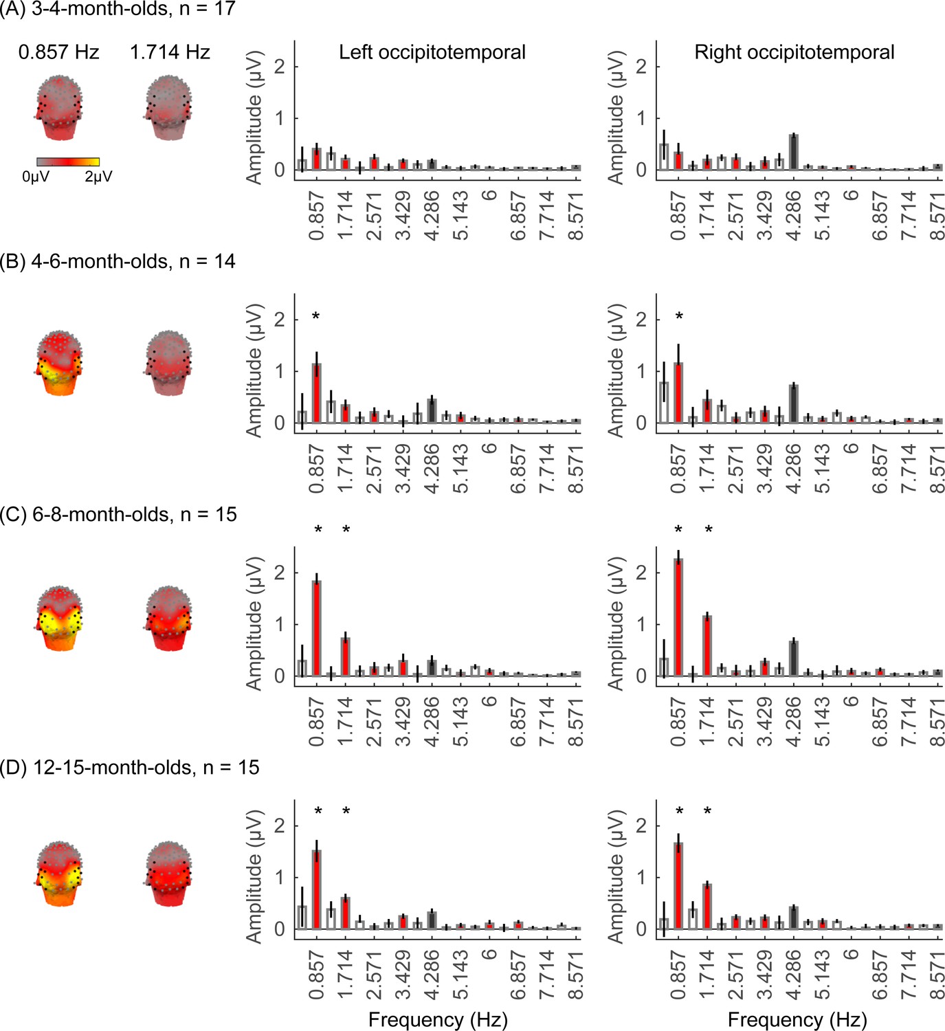
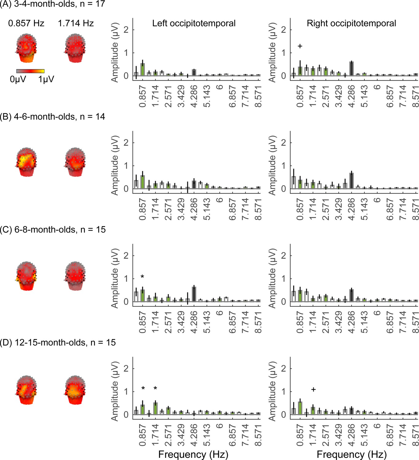
Face responses emerge over occipitotemporal electrodes after 4 months of age.
Each panel shows mean responses at the category frequency and its harmonics across infants in an age group. (A) 3- to 4-month-olds, n=17; (B) 4- to 6-month-olds; n=14; (C) 6- to 8-month-olds, n=15; (D) 12- to 15-month-olds, n=15. Left panels in each row: spatial distribution of response to category frequency at the 0.857 Hz and its first harmonic. Harmonic frequencies are indicated on the top. Right two panels in each row: mean Fourier amplitude spectrum across two regions of interest (ROIs): seven left and seven right occipitotemporal electrodes (shown in black on the left panel). Data are first averaged across electrodes in each participant and then across participants. Error bars: standard error of the mean across participants of an age group. Asterisks: significant amplitude vs. zero (p<0.05, false discovery rate [FDR] corrected at two levels). Black bars: image frequency and harmonics; colored bars: category frequency and harmonics. White bars: noise frequencies. Responses for the other categories (limbs, corridors, characters, and cars) in Appendix 1—figures 5–8.
Figure 4
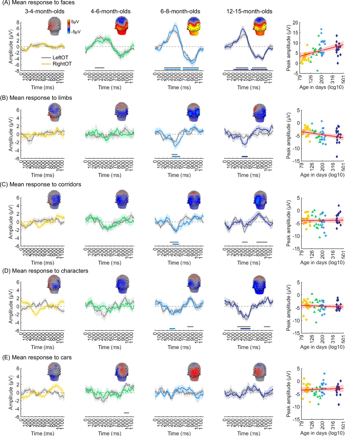
Temporal dynamics of category-selective responses as a function of age.
Category-selective responses to (A) faces, (B) limbs, (C) corridors, (D) characters, and (E) cars over left and right occipitotemporal region of interest (ROI). Data are averaged across electrodes of an ROI and across individuals. Left four panels in each row show the responses in the time domain for the four age groups. Colored lines: mean responses in the right occipitotemporal ROI. Gray lines: mean responses in the left occipitotemporal ROI. Colored horizontal lines above x-axis: significant responses relative to zero for the right OT ROI. Gray horizontal lines above x-axis: significant responses relative to zero for the left OT ROI. Top: 3D topographies of the spatial distribution of the response to target category stimuli at a 483–500 ms time window after stimulus onset. Right panel in each row: amplitude of the peak deflection defined in a 400–700 ms time interval after stimulus onset. Each dot is a participant; dots are colored by age group. Red line: linear mixed model (LMM) estimate of peak amplitude as a function of log10(age). Shaded area: 95% CI.
Figure 5
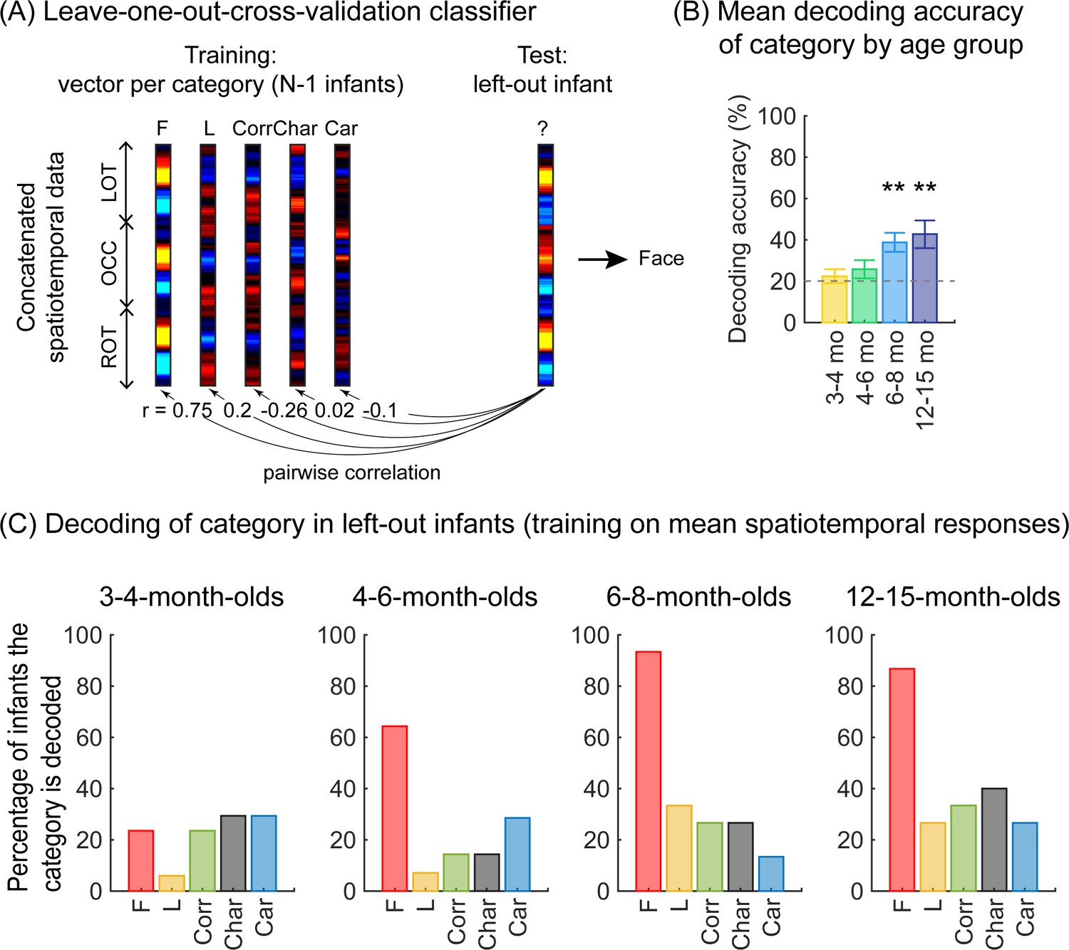
Successful decoding of faces from mean spatiotemporal responses starting from 4 months of age.
(A) An illustration of winner-takes-all leave-one-out-cross-validation (LOOCV) classifier from mean spatiotemporal response patterns of each category. Spatiotemporal patterns of response for each category are generated by concatenating the mean time courses from N–1 infants from three regions of interest (ROIs): left occipitotemporal (LOT), occipital (OCC), and right occipitotemporal (ROT). At each iteration, we train the classifier with the mean spatiotemporal patterns of each category from N–1 infants, and test how well it predicts the category the left-out infant is viewing from their spatiotemporal brain response. The winner-take-all (WTA) classifier determines the category based on the training vector that has highest pairwise correlation with the test vectors. (B) Mean decoding accuracies across all five categories in each age group. Asterisks: significant decoding above chance level (p<0.01, Bonferroni corrected, one-tailed). (C) Percentage of infants in each age group we could successfully decode for each category. Dashed lines: chance level.
Figure 6
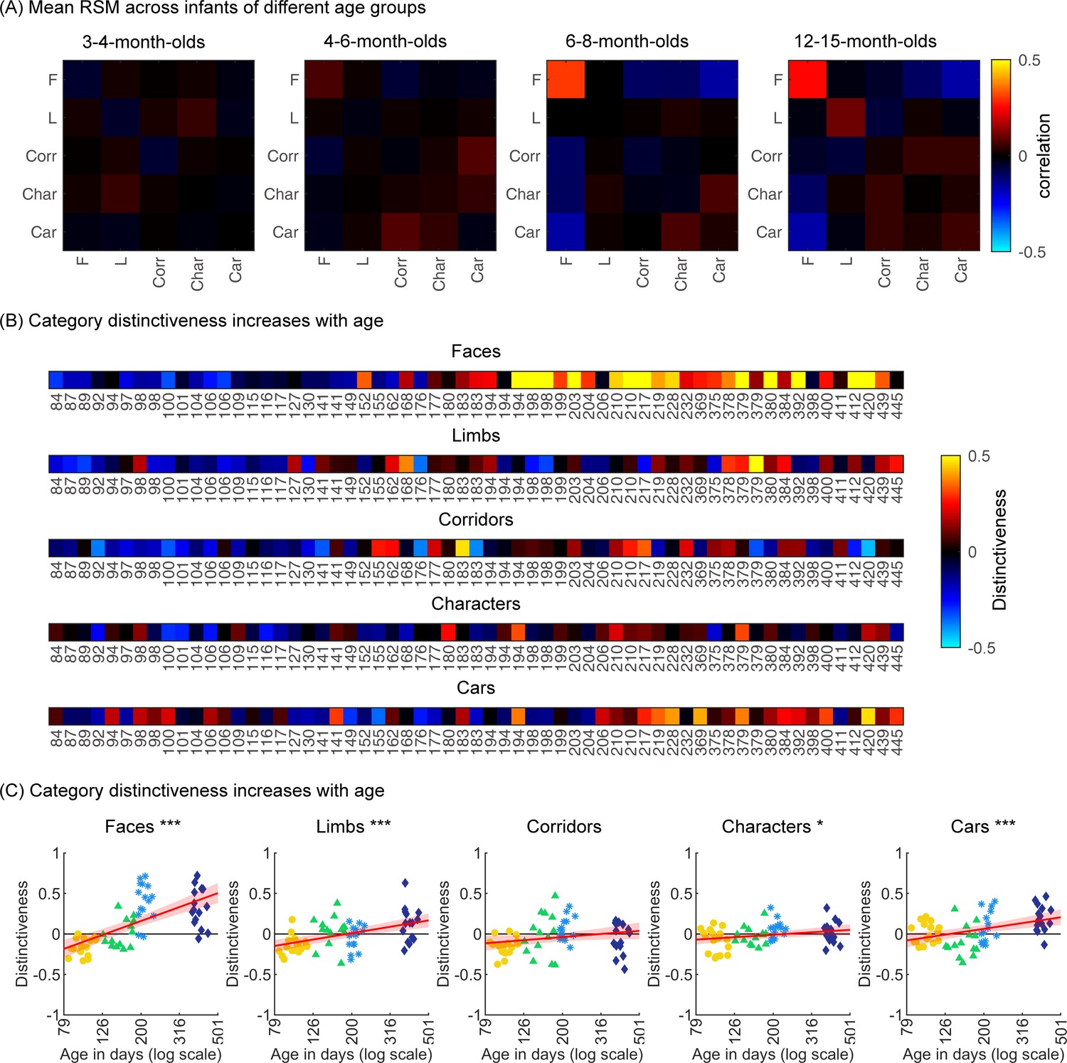
Individual split-half spatiotemporal pattern analyses reveal category information slowly emerges in the visual cortex after 6 months of age.
(A) Representation similarity matrices (RSMs) generated from odd/even split-halves of the spatiotemporal patterns of responses in individual infants. Spatiotemporal patterns for each category are generated by concatenating the mean time courses of each of 23 electrodes across left occipitotemporal (LOT), occipital (OCC), and right occipitotemporal (ROT). (B) Category distinctiveness calculated for each infant and category by subtracting the mean between-category correlation values from the within-category correlation value. (C) Distinctiveness as a function of age; panels by category; each dot is a participant. Dots are colored by age group. Red line: linear mixed model (LMM) estimates of distinctiveness as a function of log10(age). Shaded area: 95% CI.
Figure 7

Selective responses to items of a category and distinctiveness in distributed patterns develop at different times during the first year of life.
Blue arrows: presence of significant mean region of interest (ROI) category-selective responses in lateral occipital ROIs, combining results of analyses in the frequency and time domains. Yellow arrows: presence of significantly above zero distinctiveness in the distributed spatiotemporal response patterns across occipital and lateral occipital electrodes.
Appendix 1—figure 1
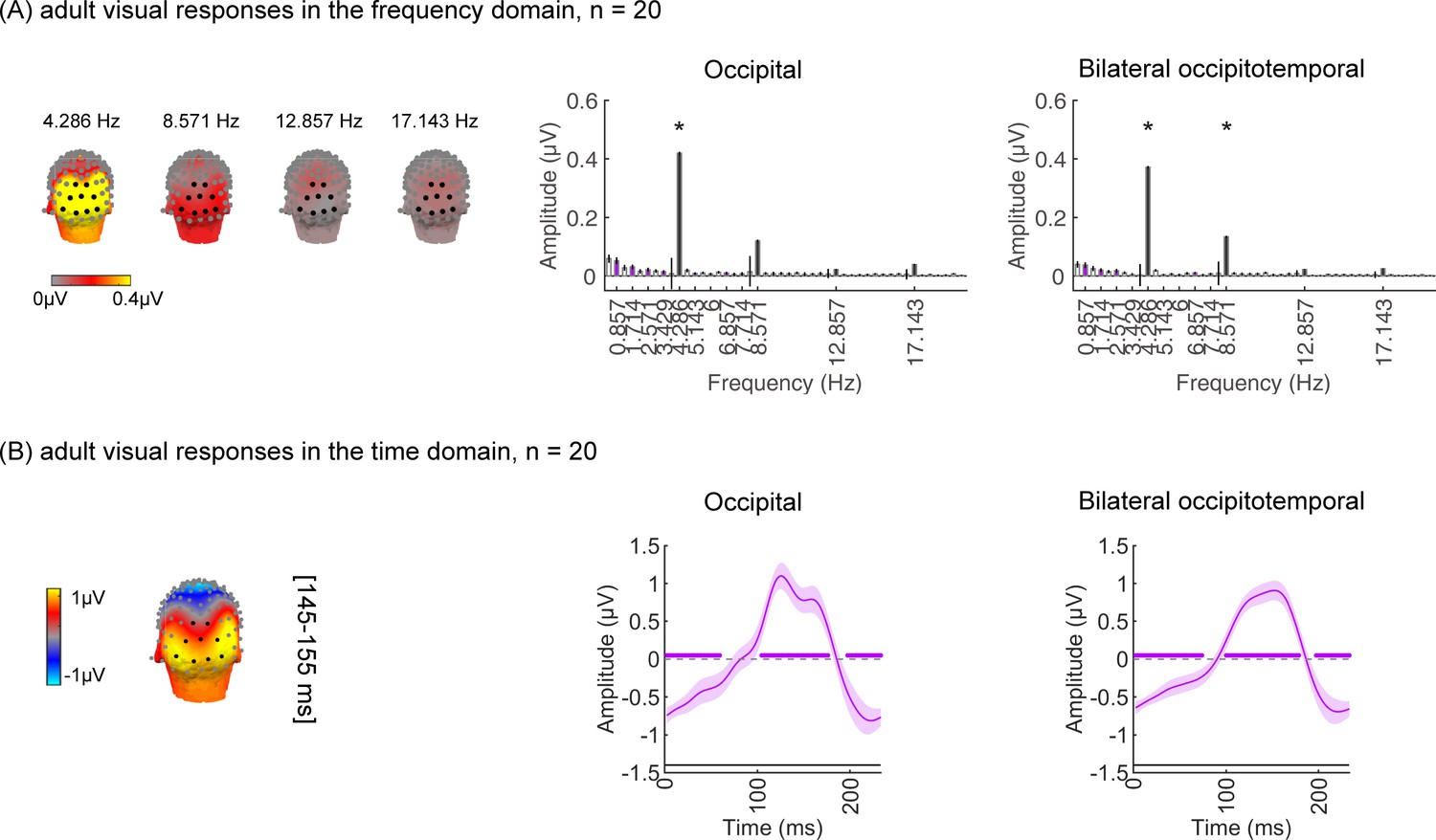
Robust visual and categorical responses recorded over occipitotemporal and occipital cortex in 20 adults.
(A) Left panel: spatial distribution of visual response at 4.286 Hz and harmonic. Harmonic frequencies are indicated on the top. Right panel: mean Fourier amplitude spectrum across 14 electrodes in the occipitotemporal and 9 electrodes in the occipital regions of interest (ROIs). Error bars: standard error of the mean across participants. Black bars: image frequency and harmonics; Purple bars: category frequency and harmonics. Asterisks: significant response amplitude from zero at pFDR<0.05. (B) Left: spatial distribution of visual responses at time window 145–155 ms. Right: Mean visual responses over two ROIs in the time domain. Waveforms are shown for a time window of 233 ms during which one image is shown. Shaded area: standard error of the mean across participants. Blank line at around y=–1.5: stimulus onset duration. To define time windows in which amplitudes were significantly different from zero, we used a cluster-based nonparametric permutation t-test (1000 permutations, with a threshold of p<0.05, two-tailed) on the post-stimulus onset time points (0–1167 ms) (Appelbaum et al., 2006; Blair and Karniski, 1993).
Appendix 1—figure 2
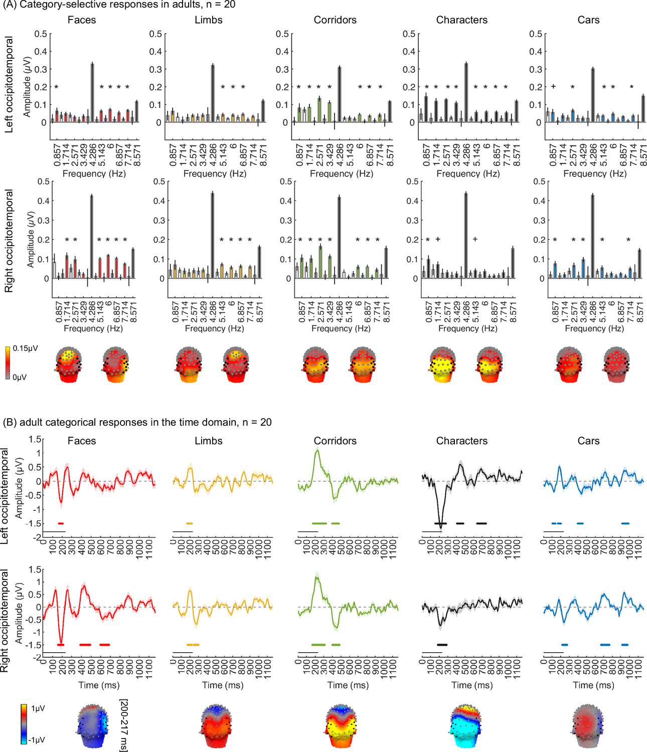
Adult control: using the same amount of data as infants reveals strong category-selective responses in adults’ occipitotemporal cortex.
(A) Mean Fourier amplitude spectrum across seven (left OT: 57, 58, 59, 63, 64, 65, 68; right OT: 90, 91, 94, 95, 96, 99) electrodes in bilateral occipitotemporal regions of interest (ROIs). Data are first averaged in each participant and then across 20 participants. Error bars: standard error of the mean across participants. Black bars: visual response at image frequency and harmonics; Colored bars: categorical response at category frequency and harmonics. Asterisks: significant response amplitude from zero at pFDR<0.05 for category harmonics. Crosses: significant response amplitude from zero at p<0.05 with no FDR correction. Black dots: ROI channels used in analysis. (B) Mean category-selective responses in the time domain. Data are averaged across electrodes of each of the left and right occipitotemporal ROI in each participant and then across participants. Colored lines along x-axis at y=–1.5: significant deflections against zero (calculated with a cluster-based method, see Methods part). Black line above x-axis: stimulus onset duration. Bottom panel: spatial distribution of category-selective responses at time window 200–217 ms.
Appendix 1—figure 3
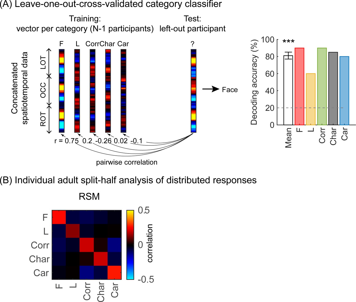
Adult control: using the same amount of data as infants reveals distributed category-selective responses in adults’ occipitotemporal cortex.
(A) Left: An illustration of winner-takes-all leave-one-out-cross-validation (LOOCV) classifier using the spatiotemporal response patterns of each category. Spatiotemporal patterns of response for each category are generated by concatenating the mean time courses from each of the three regions of interest (ROIs): left occipitotemporal (LOT), occipital (OCC), and right occipitotemporal (ROT). At each iteration, we train the classifier with the mean spatiotemporal patterns of each category from N–1 participants, and test how well it predicts the category the left-out participant is viewing from their spatiotemporal brain response. This is a winner-take-all classifier which predicts the category based on the highest pairwise correlation between the training and testing vectors. Right: White: mean decoding accuracy across all five categories. In adults, this is significantly above chance level (t(19) = 15.4, p<0.001). Colored: decoding accuracy per category. (B) Left: average adult representation similarity matrix (RSM) for odd/even splits of spatiotemporal patterns of categorical over 23 electrodes in the LOT, OCC, ROT. RSMs were generated in each participant and then averaged across all participants. Diagonal: correlation of distributed responses across different exemplars of the same category. Off-diagonal: correlations across different exemplars from different categories. Acronyms: F: faces; L: limbs; Corr: corridors; Char: characters; Car: Cars.
Appendix 1—figure 4
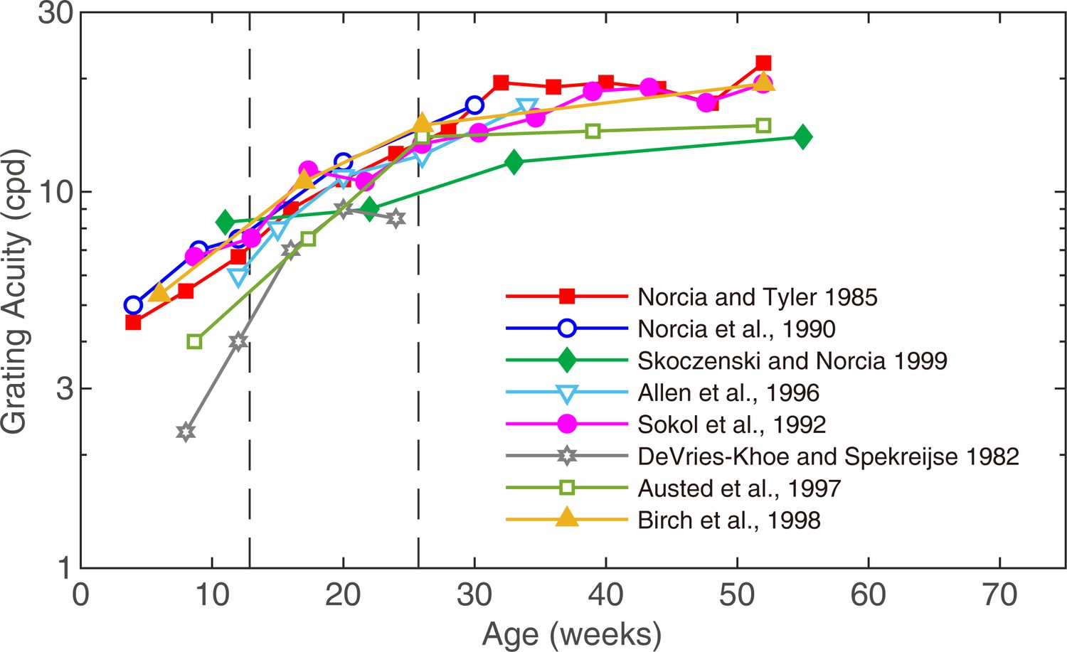
Grating acuity as a function of age measured with a swept spatial frequency technique combining electroencephalography (EEG).
(A) Acuity growth functions are similar across studies, with acuity increasing from 5 to 8 cycles per degree (cpd) in 3-month-olds to around 10–16 cpd in 6-month-olds. This figure is adapted from Norcia, 2011.
Appendix 1—figure 5
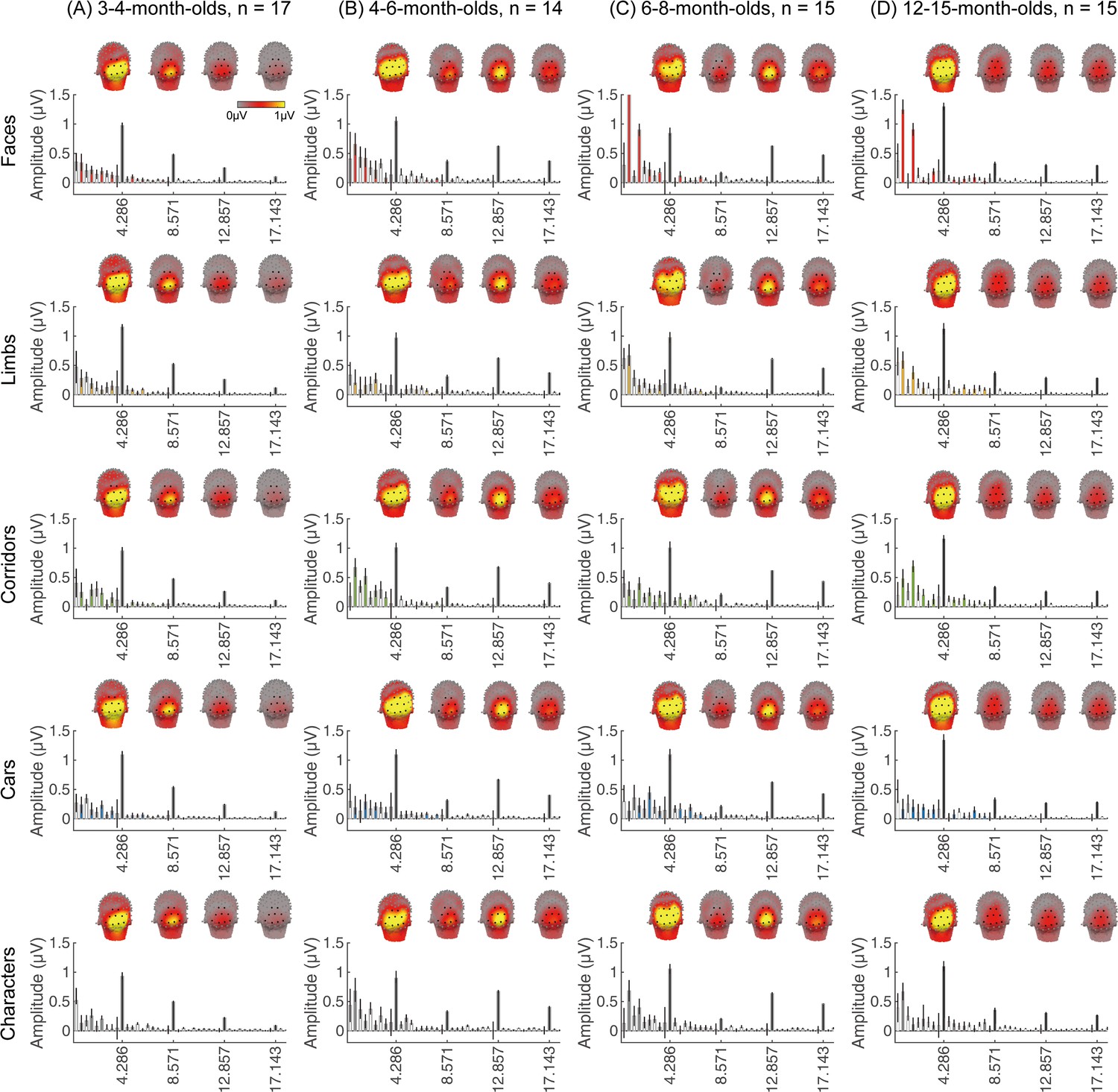
Visual responses over occipital cortex at the image-update frequency and its harmonics in five category conditions in all age groups.
Each column shows mean responses across infants in an age group for each condition. (A) 3- to 4-month-olds, n=17; (B) 4- to 6-month-olds, n=14; (C) 6- to 8-month-olds, n=15; (D) 12- to 15-month-olds, n=15. Graphs show the mean Fourier amplitude spectrum over the occipital region of interest (ROI). The visual response is at the image-update frequency (4.286 Hz) and its first three harmonics, with the mean topographies at these frequencies of interest shown on top.
Appendix 1—figure 6
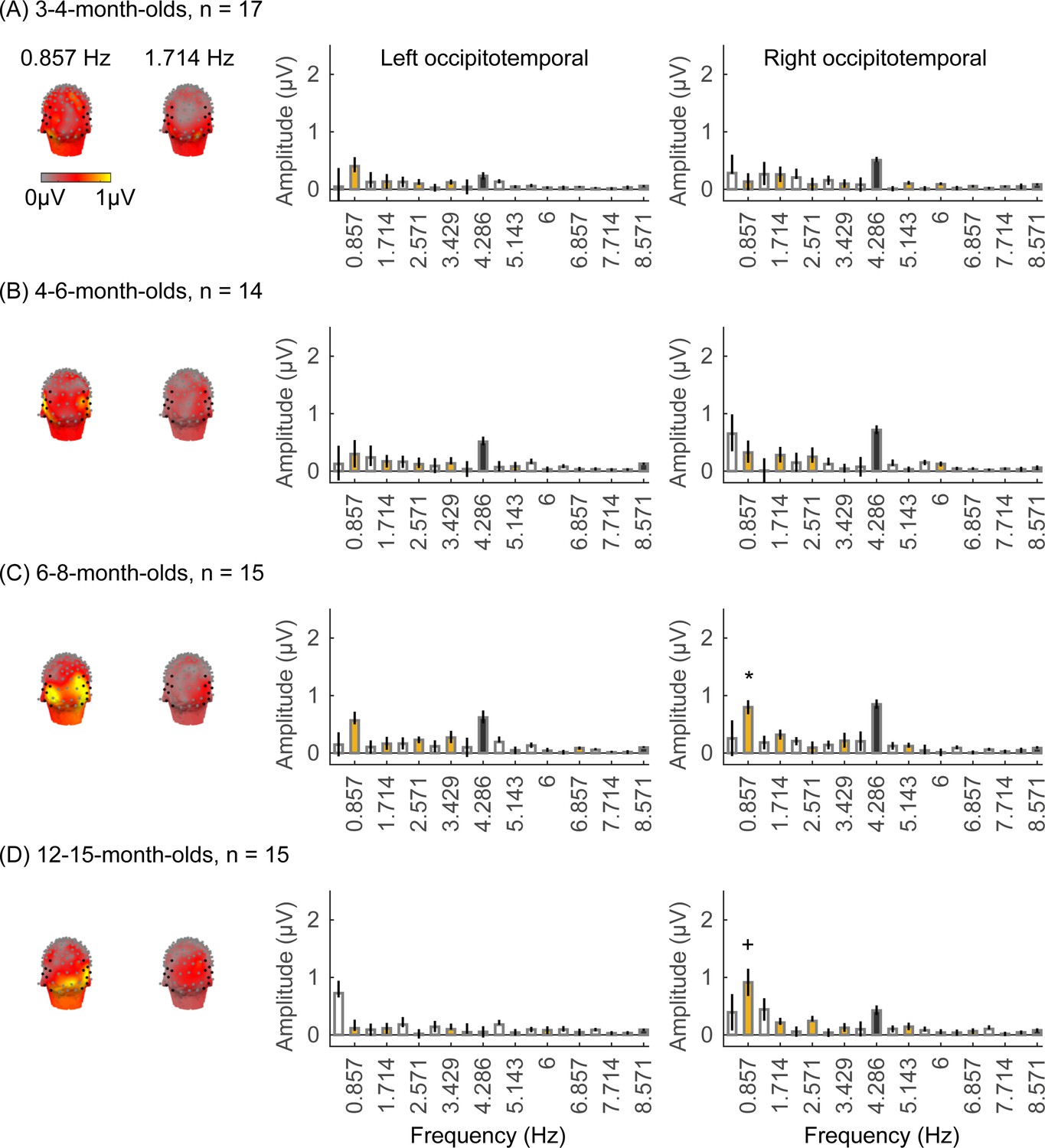
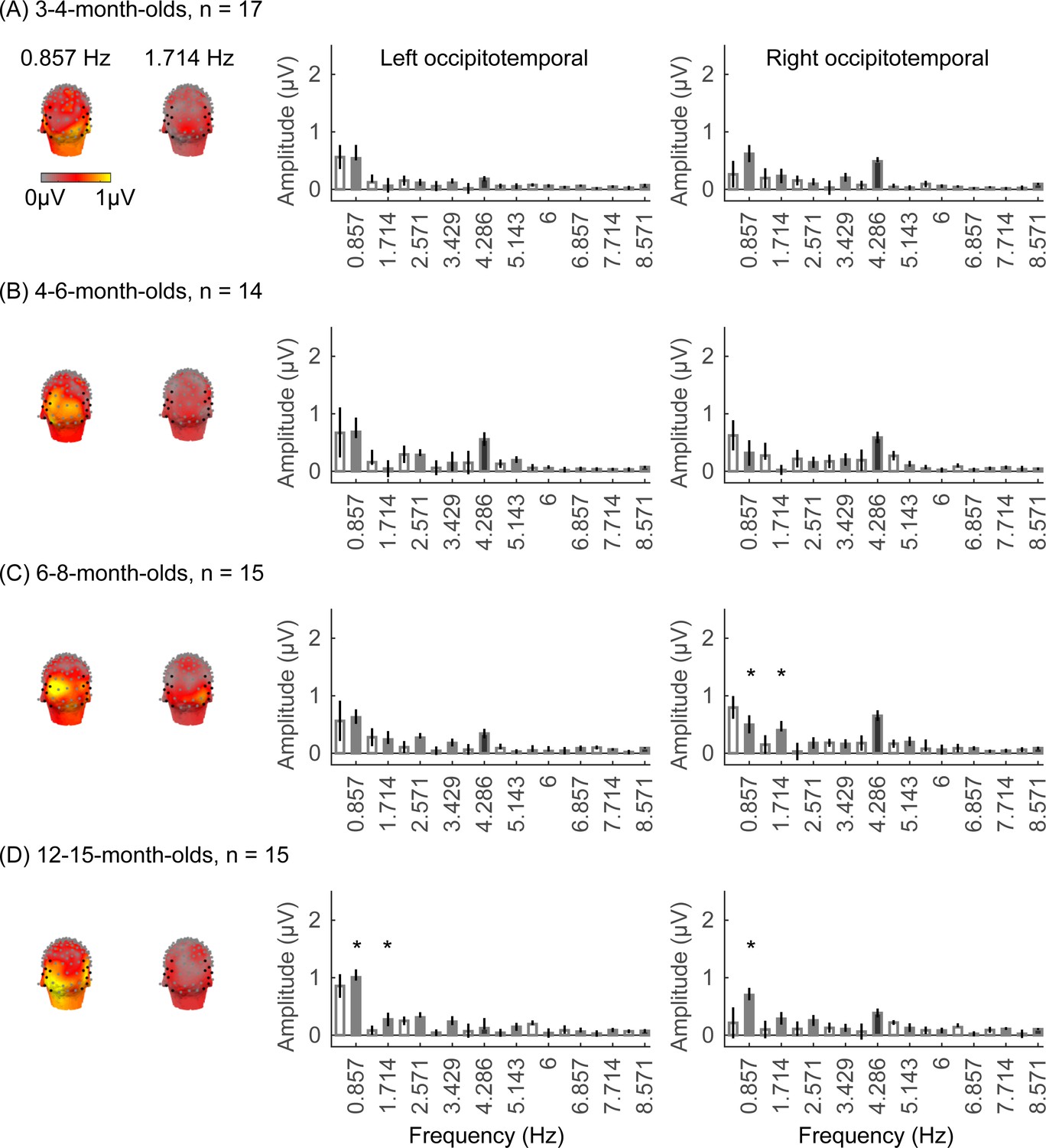
Limb responses emerge over occipitotemporal electrodes after 6 months of age.
Each panel shows mean responses at the category frequency (0.857 Hz) and its harmonics across infants in an age group. (A) 3- to 4-month-olds, n=17; (B) 4- to 6-month-olds; n=14; (C) 6- to 8-month-olds, n=15; (D) 12- to 15-month-olds, n=15. Left panels in each row: spatial distribution of categorical response at 0.857 Hz and its first harmonic. Harmonic frequencies are indicated on the top. Right two panels in each row: mean Fourier amplitude spectrum across seven left occipitotemporal electrodes and seven right occipitotemporal (shown in black on the left panel). Data are first averaged in each participant and then across participants. Error bars: standard error of the mean across participants in an age group. Asterisk: significant amplitude vs. zero (p<0.05, FDR corrected). Cross: significant amplitude vs. zero (p<0.05, with no FDR correction). Black bars: image frequency and harmonics; colored bars: category frequency and harmonics.
Appendix 1—figure 7
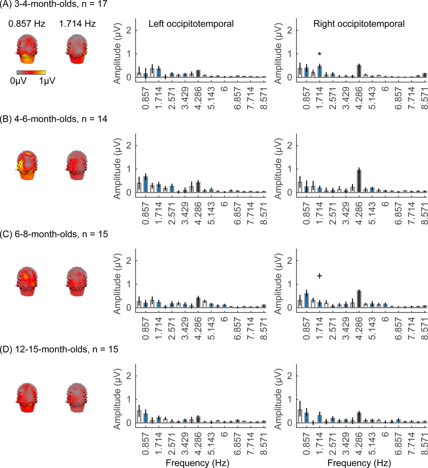
Corridor responses emerge over occipitotemporal electrodes after 6 months of age.
Each panel shows mean responses at the category frequency and its harmonics across infants in an age group. (A) 3- to 4-month-olds, n=17; (B) 4- to 6-month-olds; n=14; (C) 6- to 8-month-olds, n=15; (D) 12- to 15-month-olds, n=15. Left panels in each row: spatial distribution of categorical response at 0.857 Hz and its first harmonic. Harmonic frequencies are indicated on the top. Right two panels in each row: mean Fourier amplitude spectrum across seven left occipitotemporal electrodes and seven right occipitotemporal (shown in black on the left panel). Data are first averaged in each participant and then across participants. Error bars: standard error of the mean across participants in an age group. Asterisks: significant amplitude vs. zero (p<0.05, FDR corrected). Crosses: significant amplitude vs. zero (p<0.05, with no FDR correction). Black bars: image frequency and harmonics; colored bars: category frequency and harmonics.
Appendix 1—figure 8
Significant character responses found over occipitotemporal electrodes at 12–15 months of age.
Each panel shows mean responses at the category frequency (0.857 Hz) and its harmonics across infants in an age group. (A) 3- to 4-month-olds, n=17; (B) 4- to 6-month-olds; n=14; (C) 6- to 8-month-olds, n=15; (D) 12- to 15-month-olds, n=15. Left panels in each row: spatial distribution of categorical response at 0.857 Hz and its first harmonic. Harmonic frequencies are indicated on the top. Right two panels in each row: mean Fourier amplitude spectrum across seven left occipitotemporal electrodes and seven right occipitotemporal (shown in black on the left panel). Data are first averaged in each participant and then across participants. Error bars: standard error of the mean across participants in an age group. Asterisks: significant amplitude vs. zero (p<0.05, FDR corrected). Black bars: image frequency and harmonics; colored bars: category frequency and harmonics.
Appendix 1—figure 9
Significant car responses found over occipitotemporal electrodes at 3–4 months of age.
Each panel shows mean responses at the category frequency and its harmonics across infants in an age group. (A) 3- to 4-month-olds, n=17; (B) 4- to 6-month-olds; n=14; (C) 6- to 8-month-olds, n=15; (D) 12- to 15-month-olds, n=15. Left panels in each row: spatial distribution of categorical response at 0.857 Hz and its first harmonic. Harmonic frequencies are indicated on the top. Right two panels in each row: mean Fourier amplitude spectrum across seven left occipitotemporal electrodes and seven right occipitotemporal (shown in black on the left panel). Data are first averaged in each participant and then across participants. Error bars: standard error of the mean across participants in an age group. Asterisk: significant amplitude vs. zero (p<0.05, FDR corrected). Cross: significant amplitude vs. zero (p<0.05, with no FDR correction). Black bars: image frequency and harmonics; colored bars: category frequency and harmonics.
Appendix 1—figure 10
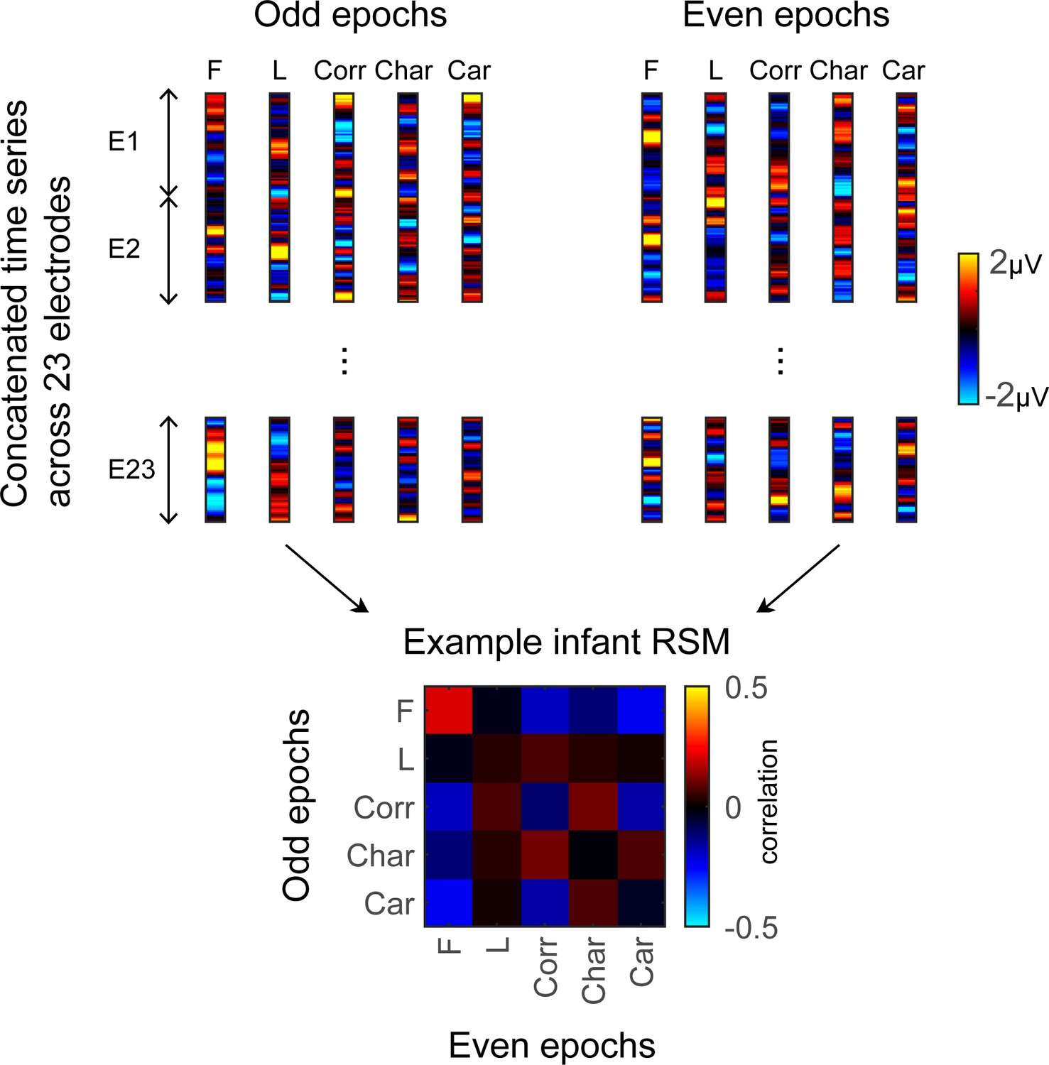
Illustration of the winner-takes-all (WTA) classifier.
In each individual, the time series data is split into odd and even trials. We concatenate the time series data from 23 electrodes in the left occipitotemporal, occipital, and right occipitotemporal regions of interest (ROIs) into a pattern vector for each split half and each condition. The classifier is trained on one half of the data (i.e. odd or even trials) and tested on how well it could predict the rest half of the data (i.e. even or odd trials) for each individual. The bottom shows the representation similarity matrix (RSM) in an example infant. Each cell indicates the correlation between distributed responses to different images of the same (on-diagonal) or different (off-diagonal) categories. F: faces; L: limbs; Corr: corridors; Char: characters; Car: cars.
Videos
Video 1
Movie showing Gaussian low-pass filtered face stimuli shown in the experiment at 5 cycles per degree (cpd).
Video 2
Movie showing Gaussian low-pass filtered limb stimuli shown in the experiment at 5 cycles per degree (cpd).
Video 3
Movie showing Gaussian low-pass filtered corridor stimuli shown in the experiment at 5 cycles per degree (cpd).
Video 4
Movie showing Gaussian low-pass filtered character stimuli shown in the experiment at 5 cycles per degree (cpd).
Video 5
Movie showing Gaussian low-pass filtered car stimuli shown in the experiment at 5 cycles per degree (cpd).
Tables
Table 1
Linear mixed models (LMMs).
| Variable | LMM formula | Results |
|---|---|---|
| Peak latency: latency of the peak waveform in each time window; window 1: 60–90 ms or window 2: 90–160 ms for 3- to 4-month-olds, and 90–110 ms for other age groups | Peak latency ~1 + log10(age in days)×time window + (1|participant) | Figure 2G. Appendix 1—table 4 |
| Peak latency ~1 + log10(age in days) + (1|participant) | Figure 2H. Appendix 1—table 5 | |
| Category-selective response amplitude: root mean square (RMS) of category-selective response at category frequency (0.857 Hz) and its first harmonic (1.714 Hz) | Response amplitude ~1 + log10(age in days)×category + (1|participant) | |
| Peak amplitude: peak response in a 400–700 ms time window | Peak amplitude ~1 + log10(age in days)×category + (1|participant) | Appendix 1—table 7 |
| Peak amplitude ~1 + log10(age in days) + (1|participant) | Figure 4. Appendix 1—table 8 | |
| Category distinctiveness of spatiotemporal responses for each of the five categories | Category distinctiveness ~log10(age in days)×category + (1|participant) | |
| Category distinctiveness ~log10(age in days) + (1|participant) | Figure 6B |
Appendix 1—table 1
Demographic information.
| 3–4 months(N=17) | 4–6 months(N=14) | 6–8 months(N=15) | 12–15 months(N=15) | |
|---|---|---|---|---|
| Age at test (days) | 84–117 | 127–183 | 194–232 | 369–445 |
| Sex | ||||
| Female | 7 | 7 | 6 | 4 |
| Male | 10 | 7 | 9 | 11 |
| Race | ||||
| White | 5 | 4 | 6 | 5 |
| Black | ||||
| Asian | 1 | 1 | 2 | |
| Mixed races | 11 | 8 | 6 | 7 |
| Unknown | 1 | 1 | 2 | 1 |
Appendix 1—table 2
Average number of valid epochs summed across all five categories for each age group before and after data pre-processing.
| 3–4 months(N=17) | 4–6 months(N=14) | 6–8 months(N=15) | 12–15 months(N=15) | Adults(N=20) | |
|---|---|---|---|---|---|
| Before pre-processing | 281 (± 103) | 270 (± 86) | 346 (± 111) | 324 (± 78) | 600 (± 0) |
| After pre-processing | 223 (± 89) | 219 (± 73) | 266 (± 91) | 269 (± 77) | 560 (± 37) |
| Ratio (after/before) | 79% | 81% | 77% | 83% | 93% |
Appendix 1—table 3
Mean (± SD) values of contrast, luminance, and similarity metrics across images within each five stimuli categories.
| Faces | Limbs | Corridors | Characters | Cars | |
|---|---|---|---|---|---|
| Contrast | 0.469 (2.533e-4) | 0.391 (3.91e-4) | 0.404 (4.04e-4) | 0.2856 (2.856e-4) | 0.3269 (3.269e-4) |
| Luminance | 0.6733 (0.0007) | 0.6729 (0.0011) | 0.6732 (0.0011) | 0.6732 (0.0008) | 0.6733 (0.0009) |
| Similarity | 0.9855 (0.0063) | 0.9555 (0.0039) | 0.9569 (0.0051) | 0.9563 (0.0033) | 0.9570 (0.0044) |
Appendix 1—table 4
Peak latency of visual responses by age and time window (window 1: 60–90 ms; window 2: 90–160 ms for 3- to 4-month-olds, and 90–110 ms for other groups).
Formula: Peak latency ~1 + log10(age) × time window + (1|participant). Significant effects are indicated by asterisks.
| Parameter | β | CI | df | t | p |
|---|---|---|---|---|---|
| Intercept | –54.61 | −100.82, –8.41 | 118 | –2.34 | 0.021* |
| Age | 39.77 | 19.51, 60.02 | 118 | 3.89 | 0.00017*** |
| Window | 141.68 | 112.92, 170.45 | 118 | 9.75 | 7.69e-17*** |
| Age×window | –45.78 | −58.39, –33.17 | 118 | –7.19 | 6.39e-11** |
Appendix 1—table 5
Peak latency of visual responses by age at each of the two time windows.
Formula: Peak latency ~1 + log10(age) + (1|participant). Significant effects are indicated by asterisks.
| Window | Parameter | β | CI | df | t | p |
|---|---|---|---|---|---|---|
| Window1 | Intercept | 90.19 | 75.66, 104.72 | 59 | 12.42 | 4.22e-18*** |
| Age | –7.44 | −13.82, –1.06 | 59 | –2.33 | 0.02* | |
| Window2 | Intercept | 218.09 | 196.05, 240.13 | 59 | 19.80 | 9.64e-28*** |
| Age | –46.91 | −56.56, –37.27 | 59 | –9.73 | 7.06e-14*** |
Appendix 1—table 6
Analysis of peak amplitude of visual responses by age and time window.
Formula: Peak amplitude ~1 + log10(age) × time window + (1|participant). Significant effects are indicated by an asterisk.
| Parameter | β | CI | df | t | p |
|---|---|---|---|---|---|
| Intercept | –18.69 | −32.35, –5.03 | 118 | –2.71 | 0.008** |
| Age | 3.93 | –2.05, 9.92 | 118 | 1.30 | 0.20 |
| Window | 17.24 | 8.66, 25.82 | 118 | 3.98 | 0.0001*** |
| Age×window | –4.90 | −8.66, –1.14 | 118 | –2.58 | 0.011* |
Appendix 1—table 7
Peak amplitude of visual responses by age at each of the two time windows.
Formula: Peak amplitude ~1 + log10(age) + (1|participant). Significant effects are indicated by asterisks.
| Window | Parameter | β | CI | df | t | p |
|---|---|---|---|---|---|---|
| Window1 | Intercept | 1.69 | –3.42, 6.79 | 59 | 0.66 | 0.51 |
| Age | 0.91 | –1.33, 3.15 | 59 | 0.82 | 0.42 | |
| Window2 | Intercept | 11.16 | 4.80, 17.51 | 59 | 3.51 | 0.0009*** |
| Age | –3.59 | −6.38, –0.81 | 59 | –2.58 | 0.012* |
Appendix 1—table 8
Analysis of peak amplitude of waveforms of category responses by age and category.
Separate linear mixed models (LMMs) were done separately for the left occipitotemporal (OT) and right OT regions of interest (ROIs). Formula: Peak amplitude ~1 + log10(age) × category + (1|participant); Peak latency ~1 + log10(age) × category + (1|participant). Significant effects are indicated by an asterisk.
| ROI/metric | Parameter | β | CI | df | t | p |
|---|---|---|---|---|---|---|
| Left OT/ | Intercept | –1.35 | –7.36, 4.66 | 301 | –0.44 | 0.66 |
| amplitude | Age | 2.62 | –0.02, 5.25 | 301 | 1.95 | 0.052 |
| Category | 0.18 | –1.58, 1.93 | 301 | 0.20 | 0.84 | |
| Age×category | –0.20 | –0.97, 0.57 | 301 | –0.51 | 0.61 | |
| Left OT/ | Intercept | 730.29 | 477.96, 982.61 | 301 | 5.70 | 2.9e-8*** |
| latency | Age | –97.17 | –207.76, 13.43 | 301 | –1.73 | 0.08 |
| Category | –43.35 | –119.43, 32.73 | 301 | –1.12 | 0.26 | |
| Age×category | 20.24 | –13.11, 53.58 | 301 | 1.19 | 0.23 | |
| Right OT/ | Intercept | –7.39 | −14.44, –0.36 | 301 | –2.07 | 0.04* |
| amplitude | Age | 5.53 | 2.45, 8.62 | 301 | 3.53 | 0.0005*** |
| Category | 2.19 | 0.06, 4.3 | 301 | 2.02 | 0.04* | |
| Age×category | –1.09 | −2.00, –0.14 | 301 | –2.26 | 0.02* | |
| Right OT/ | Intercept | 922.47 | 667.95, 1177 | 301 | 7.13 | 7.38e-12*** |
| latency | Age | –173.17 | −284.73, –61.61 | 301 | –3.05 | 0.002** |
| Category | –64.41 | –141.15, 12.33 | 301 | –1.65 | 0.10 | |
| Age×category | 28.49 | –5.15, 62.12 | 301 | 1.67 | 0.10 |
Appendix 1—table 9
Analysis of peak amplitude of waveforms of category responses for each category in the right occipitotemporal (OT) region of interest (ROI).
Formula: Peak amplitude ~age + (1|participant). Significant effects are indicated by an asterisk.
| Category | Parameter | β | CI | df | t | p |
|---|---|---|---|---|---|---|
| Faces | Intercept | –10.43 | −17.81, –3.05 | 59 | –2.83 | 0.006** |
| Age | 7.27 | 4.03, 10.51 | 59 | 4.50 | 3.30e-5*** | |
| Limbs | Intercept | 2.10 | –3.62, 7.83 | 59 | 0.74 | 0.46 |
| Age | –2.90 | −5.41,–0.38 | 59 | –2.31 | 0.02* | |
| Corridors | Intercept | –4.65 | –11.09, 1.81 | 59 | –1.44 | 0.15 |
| Age | 0.35 | –2.47, 3.18 | 59 | 0.25 | 0.80 | |
| Characters | Intercept | –2.79 | –8.06, 2.49 | 59 | –1.06 | 0.3 |
| Age | –0.66 | –2.97, 1.65 | 59 | –0.57 | 0.57 | |
| Cars | Intercept | –4.87 | –11.46, 1.73 | 59 | –1.48 | 0.15 |
| Age | 0.78 | –2.11, 3.67 | 59 | 0.54 | 0.59 |
Additional files
Download links
A two-part list of links to download the article, or parts of the article, in various formats.
Downloads (link to download the article as PDF)
Open citations (links to open the citations from this article in various online reference manager services)
Cite this article (links to download the citations from this article in formats compatible with various reference manager tools)
The emergence of visual category representations in infants’ brains
eLife 13:RP100260.
https://doi.org/10.7554/eLife.100260.3


