Multi-omics analyses and machine learning prediction of oviductal responses in the presence of gametes and embryos
- Department of OB/GYN & Women’s Health, School of Medicine, University of Missouri-Columbia, United States
- Division of Animal Sciences, College of Agriculture, Food and Natural Resources, University of Missouri-Columbia, United States
- Department of Electrical Engineering and Computer Science, College of Engineering, University of Missouri, United States
Figures
Figure 1 with 3 supplements
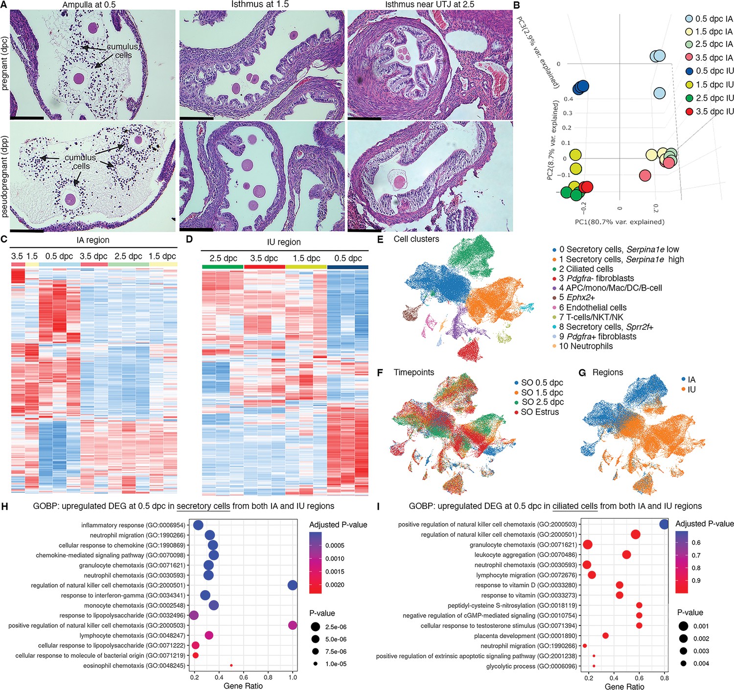
Transcriptomic analyses of the oviduct at different stages of early pregnancy.
(A) Histological analysis of different oviductal regions (ampulla, isthmus, and near the uterotubal junction (UTJ)) in mice at different stages of pregnancy (0.5, 1.5, and 2.5 dpc) and pseudopregnancy (0.5, 1.5, and 2.5 dpp) using hematoxylin and eosin (H&E) staining (scale bars = 132 μm, n = 3 mice/timepoint/region). Arrows indicate cumulus cells surrounding the eggs/fertilized eggs called cumulus–oocyte complexes. (B) Principal component analysis (PCA) of top 2500 differentially expressed genes (DEGs) identified from bulk RNA-sequencing (RNA-seq) of the infundibulum + ampulla (IA) and isthmus + UTJ (IU) regions of the oviduct collected at 0.5, 1.5, 2.5, and 3.5 dpc. Heatmap plots of unsupervised hierarchical clustering of top 2500 DEGs identified from bulk RNA-seq in the oviduct during pregnancy (0.5, 1.5, 2.5, and 3.5 dpc) of (C) IA and (D) IU regions. (E, F) Single-cell RNA-sequencing (scRNA-seq) analysis of the oviduct from superovulated (SO) estrus, SO 0.5 dpc, SO 1.5 dpc, and SO 2.5 dpc. Uniform manifold approximation and projection (UMAP) of (E) cell clusters identified from the oviduct (F) at different regions (IA and IU) and (G) at different timepoints (n = 3–4 mice/timepoint/region). Gene ontology biological processes (GOBPs) dot plots of scRNA-seq analysis when compared between upregulated DEGs from (H) secretory epithelial cells and (I) ciliated epithelial cells at SO 0.5 dpc compared to SO estrus from both IA and IU regions.
Figure 1—figure supplement 1
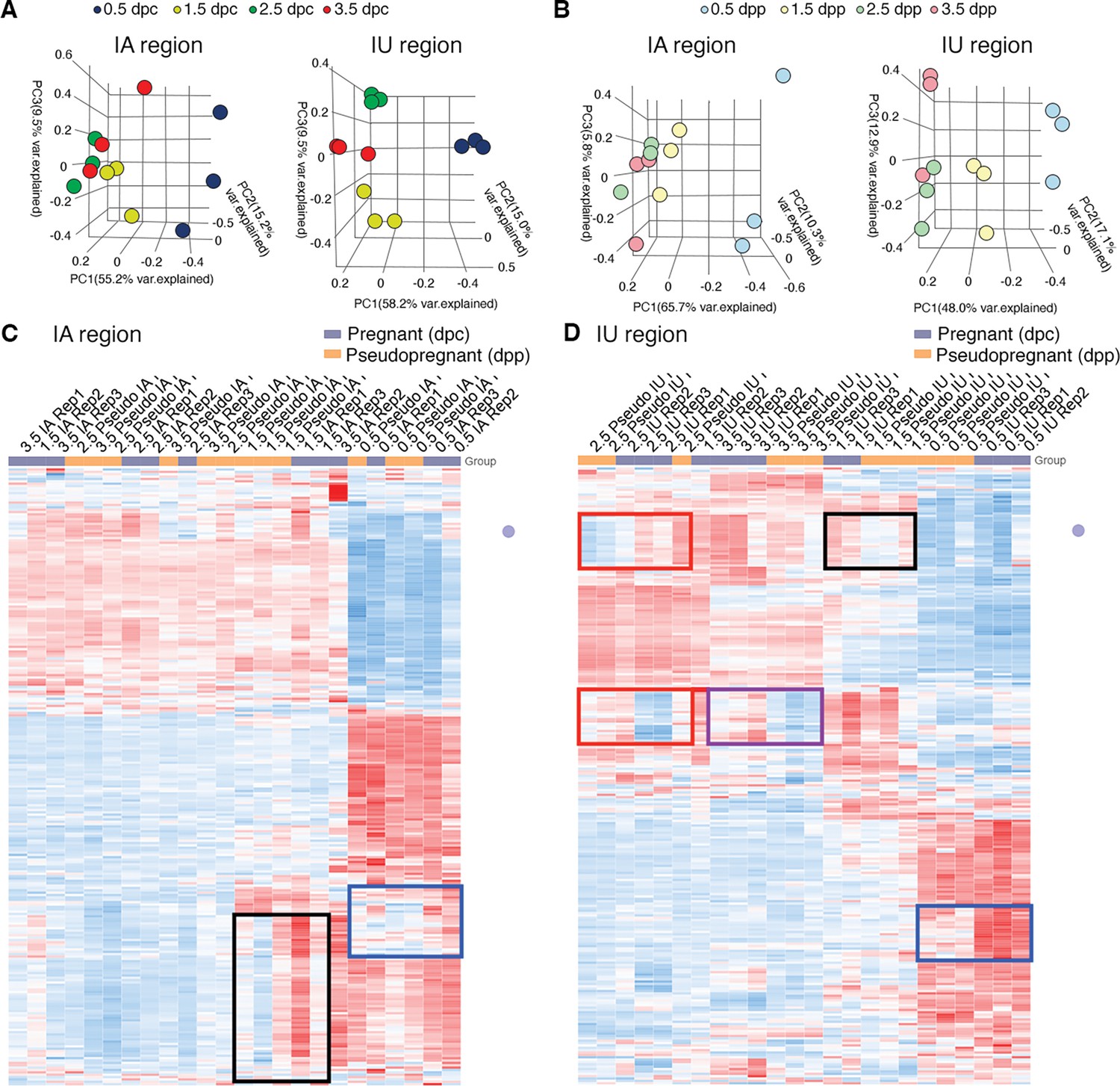
Transcriptomic profiles of mouse oviducts during pregnancy and pseudopregnancy.
Principal component analysis of top 2500 differentially expressed genes (DEGs) identified from bulk RNA-sequencing (RNA-seq) of the oviduct collected during (A) pregnancy at 0.5, 1.5, 2.5, and 3.5 days of pregnancy (dpc) and (B) pseudopregnancy at 0.5, 1.5, 2.5, and 3.5 days of pseudopregnancy (dpp). Data are separated into infundibulum–ampulla (IA) compared to isthmus–uterotubal junction (IU) regions. Heatmap plots of unsupervised hierarchical clustering of top 2500 DEGs in the oviduct during pregnancy (0.5, 1.5, 2.5, and 3.5 dpc) compared to pseudopregnancy (0.5, 1.5, 2.5, and 3.5 dpp) of (C) IA and (D) IU regions. Gene expression patterns that differ between 0.5 dpc (blue boxes), 1.5 dpc (black boxes), 2.5 dpc (red boxes), and 3.5 dpc (purple box) compared to the corresponding dpp (n = 3 mice/timepoint/region). Blue: downregulated, red: upregulated.
Figure 1—figure supplement 2
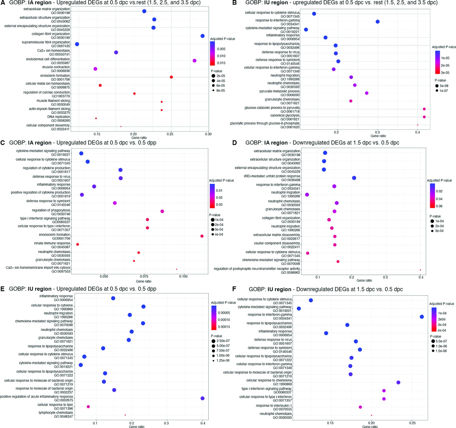
Dot Plots of biological processes from gene ontology (GOBP) analysis from differentially expressed genes (DEGs) from bulk RNA-sequencing (RNA-seq) analysis at different timepoints.
GOBP that were upregulated at 0.5 dpc compared to 1.5–3.5 dpc (0.5 dpc vs. rest) in (A) IA and (B) IU regions. GOBP that were (C) upregulated at 0.5 dpc compared to 0.5 dpp and (D) downregulated at 1.5 dpc compared to 0.5 dpc in the (C, D) IA region or (E, F) IU region, respectively. Gene ontology (GO) numbers were indicated within graphs. Gene ratio indicates the ratio of genes that were present in our dataset compared to all genes in the database for each BP.
Figure 1—figure supplement 3
Analyses of differentially expressed genes that were enriched at different timepoints.
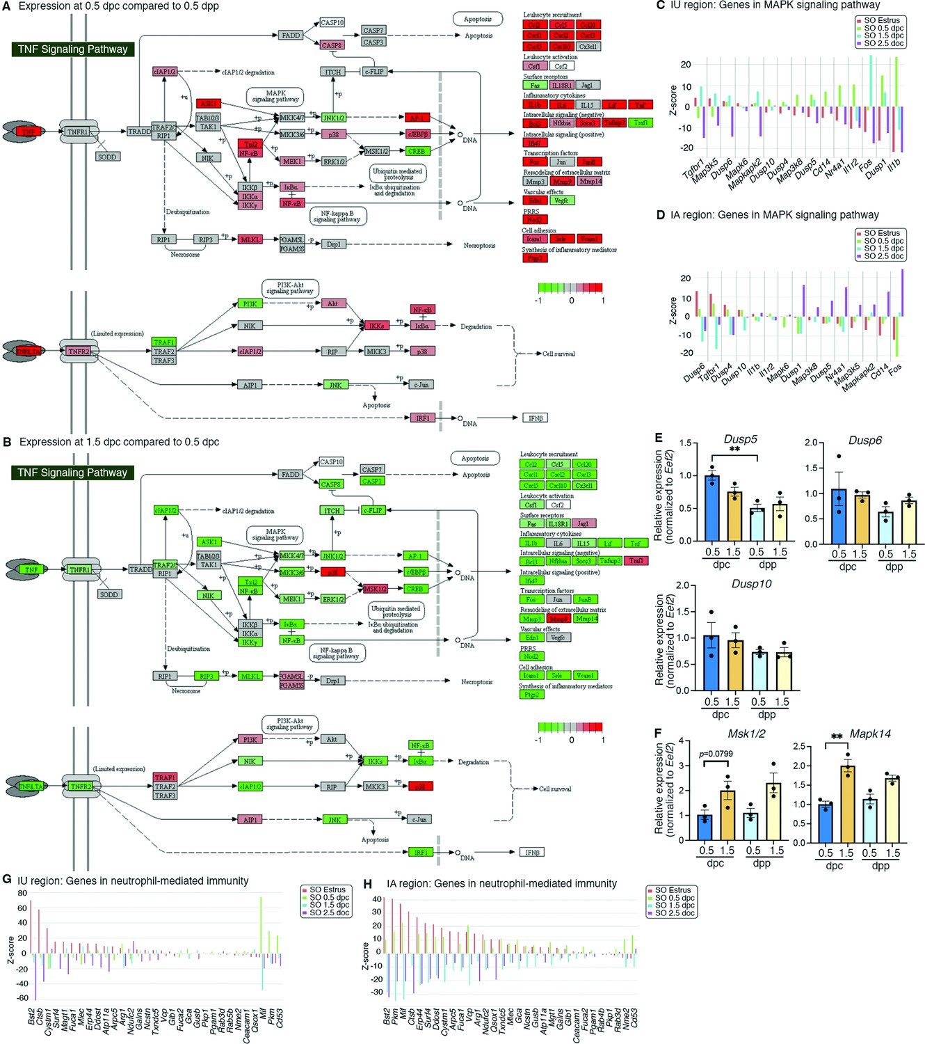
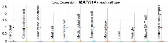
KEGG pathway analysis of genes from bulk RNA-sequencing (RNA-seq) data in the TGF signaling pathway at (A) 0.5 dpc compared to 0.5 dpp and at (B) 1.5 dpc compared to 0.5 dpc. Expression of genes in the mitogen-activated protein kinase (MAPK) signaling pathways in single-cell RNA-sequencing (scRNA-seq) dataset in the (C) IU and (D) IA regions. qPCR validation of (E) Dusp5, Dusp6, and Dusp10 and (F) Mak1/2 and Mapk14 in the whole oviduct at 0.5 dpc, 1.5 dpc, 0.5 dpp, and 1.5 dpp (n = 3 mice/timepoint). **p < 0.01 compared to 0.5 dpc, unpaired t-test. Expression of genes in the neutrophil-mediated immunity in scRNA-seq dataset in the (G) IU and (H) IA regions.
Figure 2 with 1 supplement
Analyses of protein abundance in the oviduct luminal fluid at different stages of pregnancy compared to Estrus.
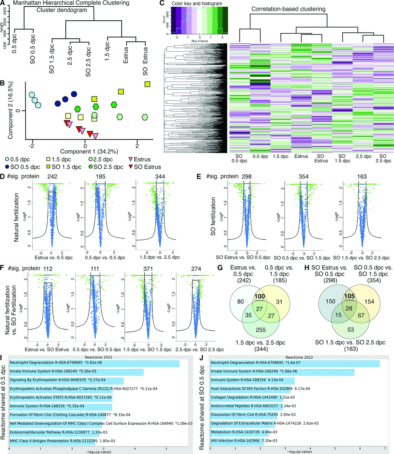
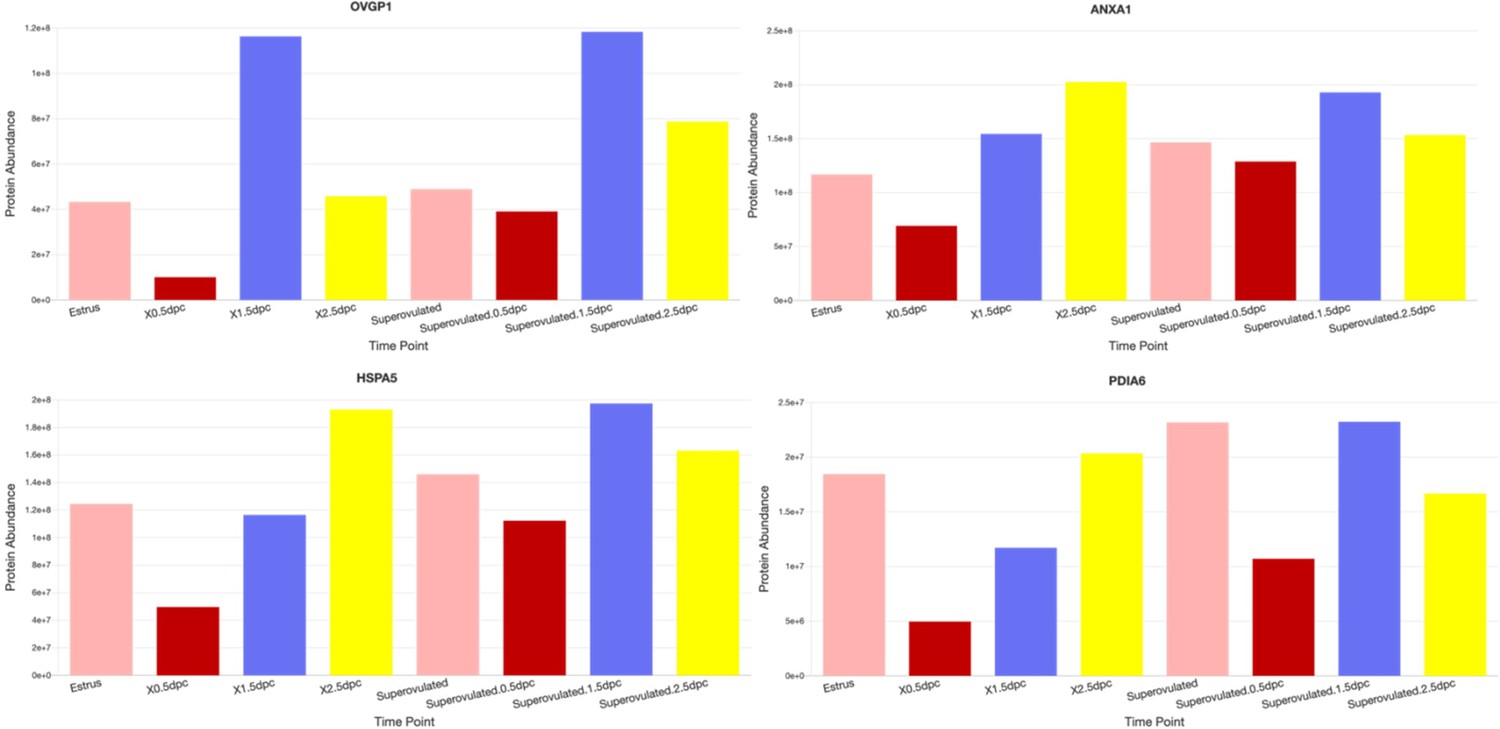
(A) Manhattan hierarchical complete clustering dendrogram of natural (estrus, 0.5 dpc, 1.5 dpc, and 2.5 dpc) and superovulated (SO estrus, SO 0.5 dpc, SO 1.5 dpc, and SO 2.5 dpc) datasets (n = pooled of 3 biological samples/timepoint). (B) Principal component analysis (PCA) plot of all datasets generated utilizing Perseus software after integration of the Gaussian transformation. (C) Correlation-based hierarchal clustering of all protein abundance. Volcano plots of significantly different protein abundances when compared between (D) natural fertilization, (E) SO fertilization, and (F) natural fertilization versus SO fertilization. Numbers of significant proteins were listed above the volcano plots. Gaussian transformed Perseus two-tailed t-tests of differentially abundant proteins in oviductal fluid at different stages during (G) natural fertilization and (H) SO fertilization. Differentially abundant proteins shared between estrus and 0.5 dpc (100) or SO estrus and SO 0.5 dpc (105) were underlined. Enricher Reactome pathway analysis of differentially abundant proteins shared at (I) 0.5 and (H) SO 0.5 dpc.
Figure 2—figure supplement 1
Enricher Reactome pathway analysis of differentially expressed proteins in the luminal fluid at (A) 1.5 and (B) 2.5 dpc.
Figure 3
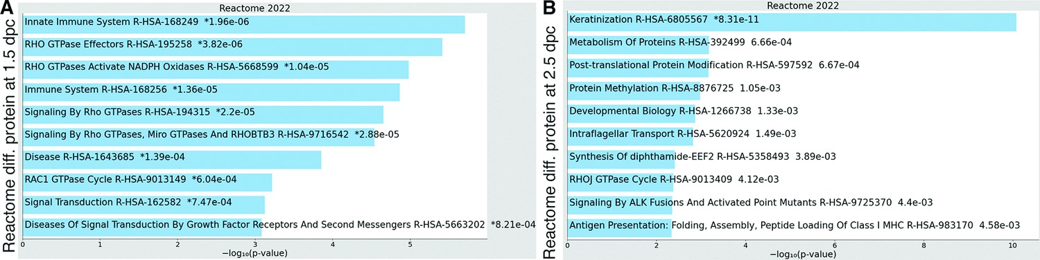
In vivo validation of RNA and proteins identified from bulk RNA-sequencing (RNA-seq) and single-cell RNA-sequencing (scRNA-seq) analysis.
(A, B) Expression of Tlr2, Ly6g, and Ptprc in the isthmus and uterotubal junction (UTJ) regions at 0.5 dpc, 1.5 dpc, 0.5 dpp, and 1.5 dpp. Scale bar = 50 μm for all images in the panel. (B) Quantification of fluorescent signal from images in (A) using FIJI software. Graph represent mean ± SEM, n = 3 mice/timepoint/region. *,**p < 0.05 or 0.01 respecitvely compared to 0.5 dpc, unpaired t-test. (C) Immunofluorescent staining of NFκB in the isthmus regions of the oviducts at 0.5 dpc, 1.5 dpc, 0.5 dpp, and 1.5 dpp. Scale bar = 50 μm for all images in the panel. (D) Quantification of fluorescent signal from images in (C) using FIJI software. Violin plots represent all measurements, n = 3 mice/timepoint/region, ****p < 0.001 compared to 0.5 dpc, unpaired t-test. (E) Immunoblotting of phosphorylated p38 and total p38 in the whole oviduct collected at 0.5 dpc, 0.5 dpp, 1.5 dpc, and 1.5 dpp. (F) Violin plots of the quantification of band intensity represented as phosphor-p38/total p38 ratio (n = 3 mice/timepoint/region). *p < 0.05 compared to 0.5 dpc, unpaired t-test. (G) IL1β ELISA of protein from the whole oviduct at 0.5 dpc, 1.5 dpc, 0.5 dpp, and 1.5 dpp (n = 3 mice/timepoint/region).
-
Figure 3—source data 1
Original files for western blot analysis displayed in Figure 3E.
- https://cdn.elifesciences.org/articles/100705/elife-100705-fig3-data1-v1.zip
-
Figure 3—source data 2
PDF file containing original western blots for Figure 3E, indicating the relevant bands and timepionts.
- https://cdn.elifesciences.org/articles/100705/elife-100705-fig3-data2-v1.zip
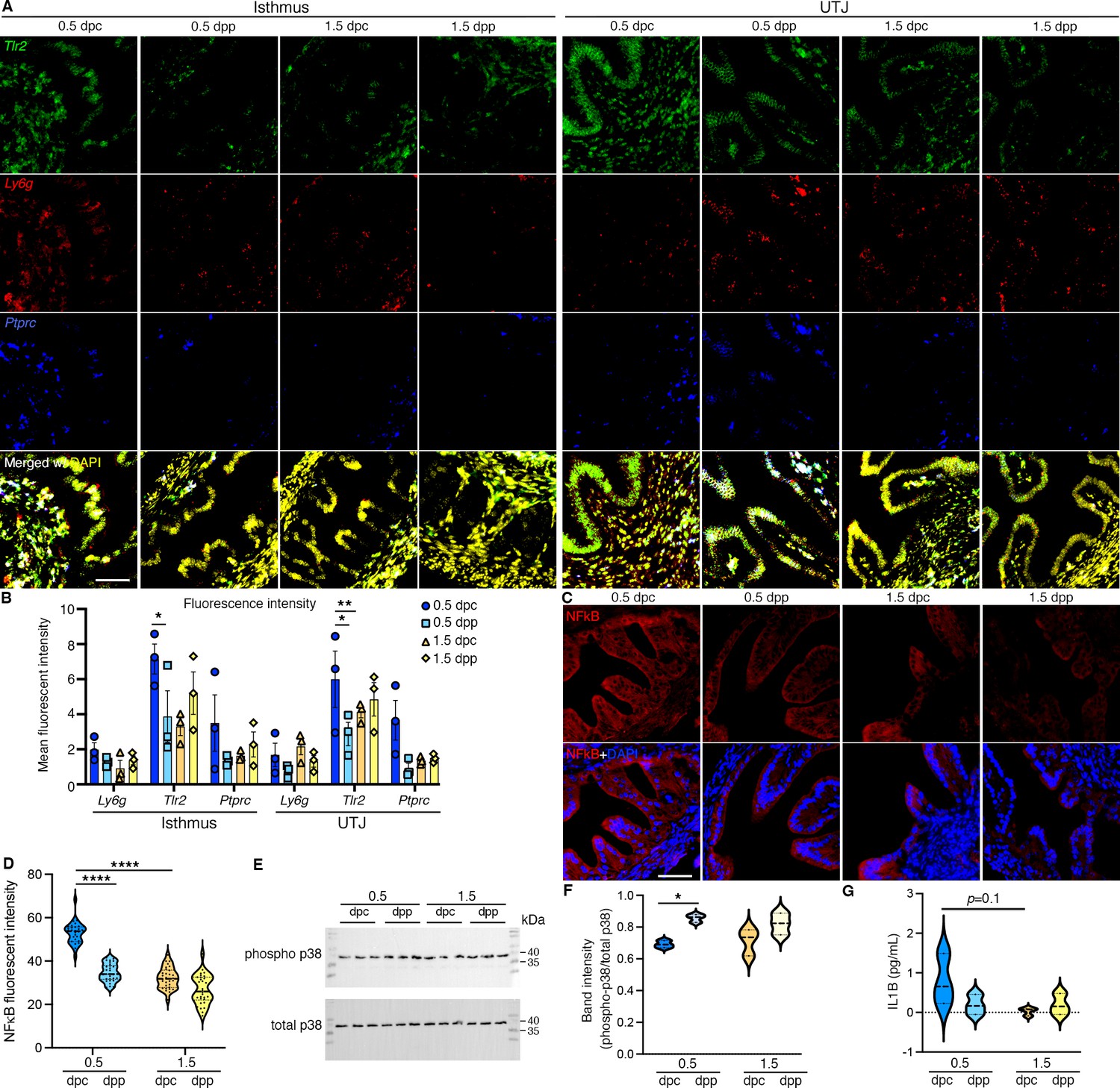
Figure 4
Overall architecture of the transformer-based model to predict proteomic abundance from bulk RNA-sequencing (RNA-seq) data of natural fertilization of oviduct.
(A) Preprocessing steps using bulk RNA-seq count per million (cpm) normalization to calculate expression values. The transformer model is equipped with a single-layer transformer encoder featuring a single-head (1-Head) self-attention mechanism to predict the abundancy of proteins (abundant or not) from the input RNA-seq data. ‘Head’ refers to blocks, modules, or connections that perform specific tasks in neural networks. A specific threshold of 0.6/0.8 was defined to label proteins as high abundance or low abundance. The Multi-Layer Perceptron (MLP) Head refers to the output layer, which is designed to perform a classification task. In this model, The MLP layer uses a multi-layer perceptron or linear layer as the backbone to divide high abundance and low abundance based on the importance or attention weights given by the previous transformer layer. (B) The visual representation of a method to extract the top 25 TFs for differential significant proteins. DGE: differential gene expression, DPA: differential protein abundance, TF: transcription factor.
Figure 5
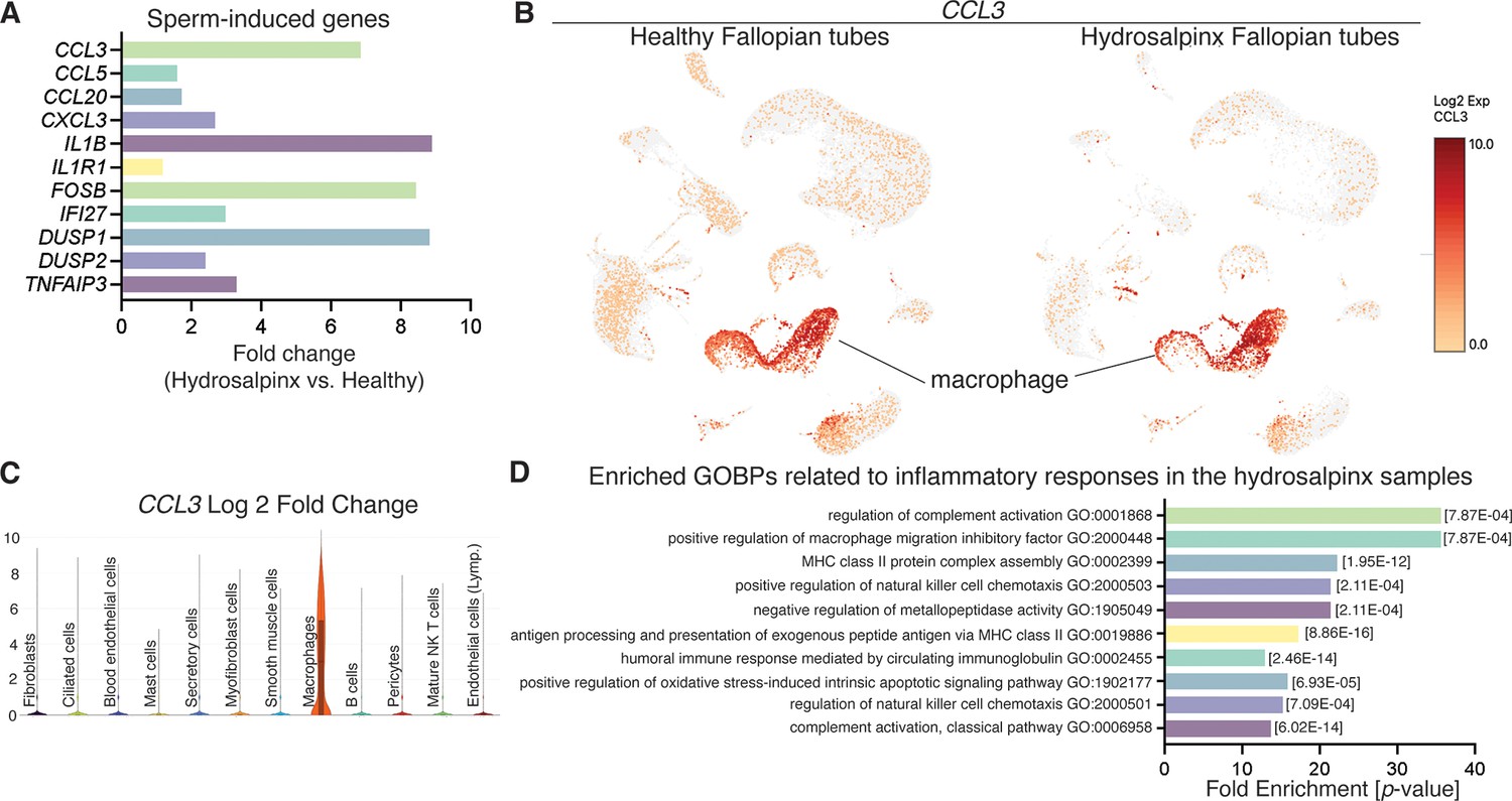
Reanalysis of data from Ulrich et al., 2022 using hydrosalpinx versus healthy Fallopian tube samples from GSE178101.
(A) Expression of sperm-induced genes identified from this current study in the hydrosalpinx compared to healthy Fallopian tube samples. (B) Uniform manifold approximation and projection (UMAP) of CCL3 in healthy and hydrosalpinx Fallopian tubes in the macrophage populations. (C) Log2foldchange of CCL3 in a violin plot comparing hydrosalpinx versus healthy Fallopian tubes. (D) Enriched gene ontology biological processes (GOBPs) related to inflammatory responses in the hydrosalpinx samples.
Figure 6
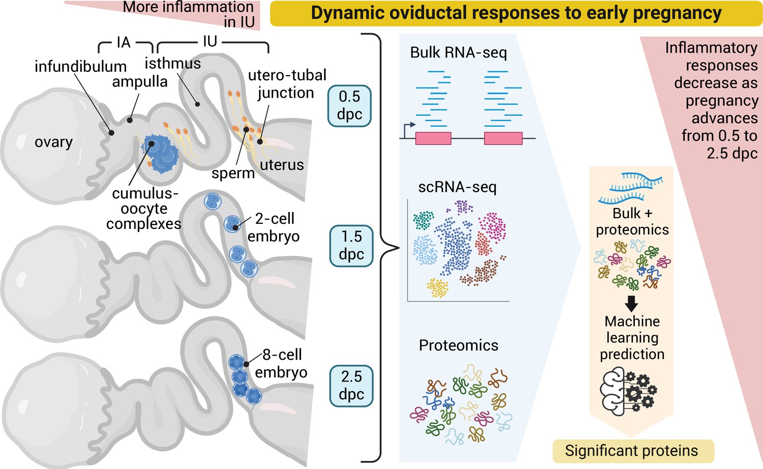
Dynamic oviductal response to early pregnancy in mice.
Bulk RNA, scRNA-sequencing, and LC–MS/MS analyses were performed using the oviductal samples collected from mice at 0.5 days post coitus (dpc) through 2.5 dpc. Data were integrated and processed using machine learning to identify potential proteins crucial during each stage of early pregnancy. Created using BioRender.
Author response image 1

Author response image 2
Author response image 3
Additional files
-
Supplementary file 1
Differential gene expression analysis from estrus.
We first performed differential gene expression (DGE) in estrus and extracted significant proteins (protein-coding genes). Then, the significant proteins were used to extract top 25 transcription factors (TFs) influencing those proteins. For DEG, FDR threshold was set to <0.05 and log2foldchange of >0.1. Enrichr Reactome and GO biological process (BP) were used to determine the enriched pathways from the TFs and influenced proteins (IPs). Each excel file contains a table with Column names or header names being significant proteins in worksheet named ‘AllTfs_diffcodinggene_sample’; rows 2–26 represent the top 25 transcription factors (TFs) influencing the corresponding protein abundance in row 1.
- https://cdn.elifesciences.org/articles/100705/elife-100705-supp1-v1.xlsx
-
Supplementary file 2
Differential gene expression analysis between the estrus and 0.5 dpc.
We first performed differential gene expression (DGE) between Control (Estrus) and timepoints and extracted significant proteins (protein-coding genes). Then, the significant proteins were used to extract top 25 transcription factors (TFs) influencing those proteins. For DEG, FDR threshold was set to <0.05 and log2foldchange of >0.1. Enrichr Reactome and GO biological process (BP) were used to determine the enriched pathways from the TFs and influenced proteins (IPs). Each excel file contains a table with Column names or header names being significant proteins in worksheet named ‘AllTfs_diffcodinggene_sample’; rows 2–26 represent the top 25 transcription factors (TFs) influencing the corresponding protein abundance in row 1.
- https://cdn.elifesciences.org/articles/100705/elife-100705-supp2-v1.xlsx
-
Supplementary file 3
Differential gene expression analysis between the estrus and 1.5 dpc.
We first performed differential gene expression (DGE) between Control (Estrus) and timepoints and extracted significant proteins (protein-coding genes). Then, the significant proteins were used to extract top 25 transcription factors (TFs) influencing those proteins. For DEG, FDR threshold was set to <0.05 and log2foldchange of >0.1. Enrichr Reactome and GO biological process (BP) were used to determine the enriched pathways from the TFs and influenced proteins (IPs). Each excel file contains a table with Column names or header names being significant proteins in worksheet named ‘AllTfs_diffcodinggene_sample’; rows 2–26 represent the top 25 transcription factors (TFs) influencing the corresponding protein abundance in row 1.
- https://cdn.elifesciences.org/articles/100705/elife-100705-supp3-v1.xlsx
-
Supplementary file 4
Differential gene expression analysis between the estrus and 2.5 dpc.
We first performed differential gene expression (DGE) between Control (Estrus) and timepoints and extracted significant proteins (protein-coding genes). Then, the significant proteins were used to extract top 25 transcription factors (TFs) influencing those proteins. For DEG, FDR threshold was set to <0.05 and log2foldchange of >0.1. Enrichr Reactome and GO biological process (BP) were used to determine the enriched pathways from the TFs and influenced proteins (IPs). Each excel file contains a table with Column names or header names being significant proteins in worksheet named ‘AllTfs_diffcodinggene_sample’; rows 2–26 represent the top 25 transcription factors (TFs) influencing the corresponding protein abundance in row 1.
- https://cdn.elifesciences.org/articles/100705/elife-100705-supp4-v1.xlsx
-
Supplementary file 5
Differential gene expression analysis between hydrosalpinx versus healthy Fallopian tubes from PMID: 35320732 (GSE178101).
We first performed differential expressed genes using Loupe Browser. Then, the significant genes were used to determine the GO biological process (BP).
- https://cdn.elifesciences.org/articles/100705/elife-100705-supp5-v1.xlsx
-
Supplementary file 6
scRNA-seq web output summary and predicted protein abundance by the transformer model.
(A) scRNA-seq output for each dataset in this study. (B) The result of predicting protein abundance from bulk RNA-seq data at 2.5 dpc by the transformer model. The model is used to classify proteins into two categories, abundant or not abundant, according to two different thresholds: 0.6 and 0.8, respectively. The model can rather accurately predict the abundant proteins from RNA-seq data.
- https://cdn.elifesciences.org/articles/100705/elife-100705-supp6-v1.pdf
-
MDAR checklist
- https://cdn.elifesciences.org/articles/100705/elife-100705-mdarchecklist1-v1.docx
Download links
A two-part list of links to download the article, or parts of the article, in various formats.
Downloads (link to download the article as PDF)
Open citations (links to open the citations from this article in various online reference manager services)
Cite this article (links to download the citations from this article in formats compatible with various reference manager tools)
Multi-omics analyses and machine learning prediction of oviductal responses in the presence of gametes and embryos
eLife 13:RP100705.
https://doi.org/10.7554/eLife.100705.3


