Aberration correction in long GRIN lens-based microendoscopes for extended field-of-view two-photon imaging in deep brain regions
- Optical Approaches to Brain Function Laboratory, Istituto Italiano di Tecnologia, Italy
- Neural Coding Laboratory, Istituto Italiano di Tecnologia, Italy
- Department of Neuroscience and Carney Institute for Brain Science, Brown University, United States
- Neural Computation Laboratory, Center for Neuroscience and Cognitive Systems @UniTn, Istituto Italiano di Tecnologia, Italy
- Biological and Environmental Sciences and Engineering Division (BESE), King Abdullah University of Science and Technology (KAUST), Saudi Arabia
- Institute for Neural Information Processing, Center for Molecular Neurobiology (ZMNH), University Medical Center Hamburg-Eppendorf (UKE), Germany
Figures
Figure 1 with 3 supplements
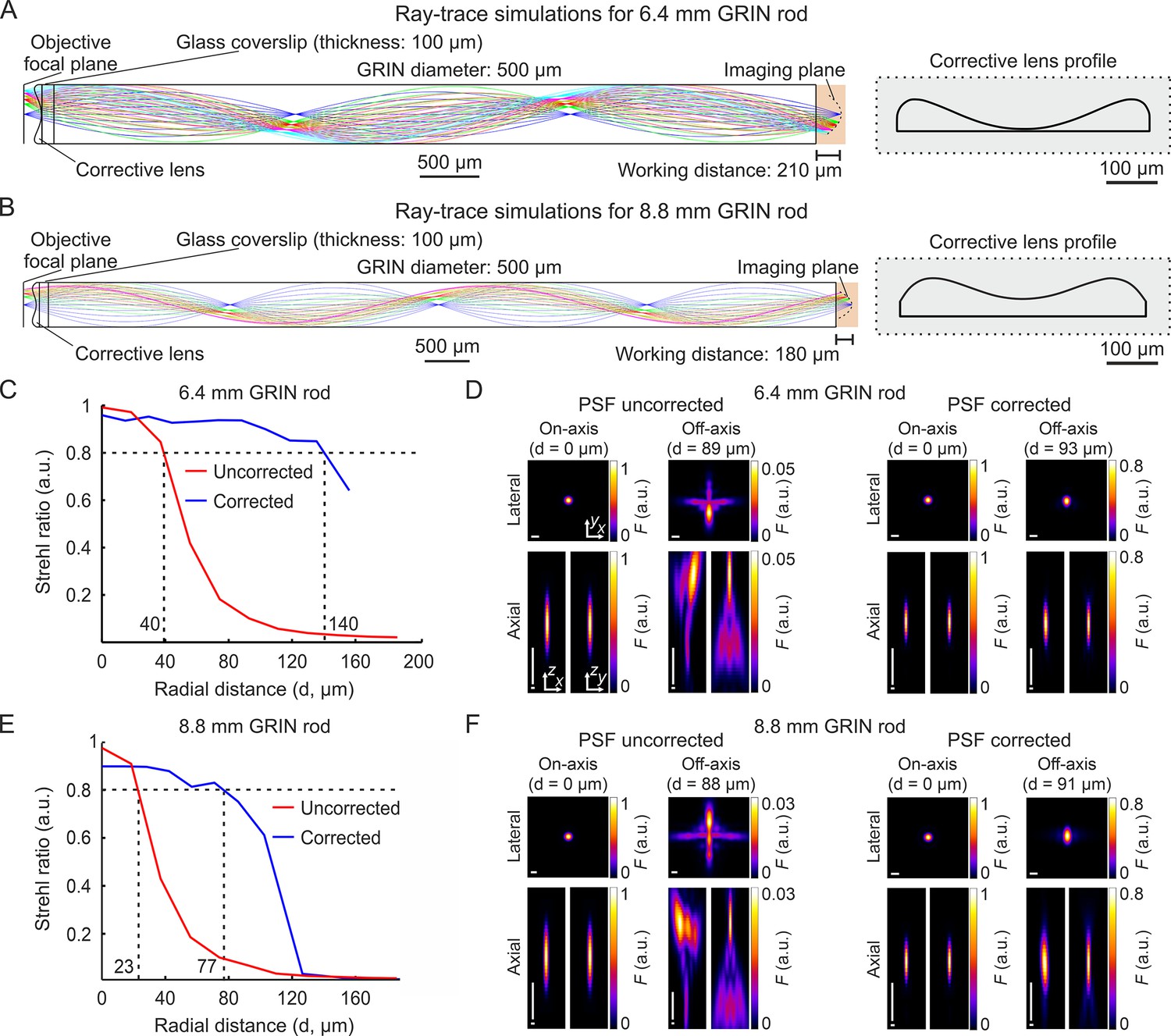
Optical simulations of long corrected microendoscopes.
(A) Ray-trace simulation for the microendoscope based on the 6.4 mm-long GRIN rod. Left: rays of 920 nm light are relayed from the objective focal plane to the imaging plane. Labels indicate geometrical parameters of the microendoscope components. Right: profile of the corrective aspherical lens that maximizes the microendoscope FOV in the optical simulation shown on the left. (B) Same as (A) for the microendoscope based on the 8.8 mm-long GRIN rod. (C,D) Optical performance of simulated microendoscope based on the 6.4 mm-long GRIN rod. (C) Strehl ratio as a function of the field radial distance (zero indicates the optical axis) computed on the focal plane in the object space (after the GRIN rod) for the corrected (blue) and the uncorrected (red) microendoscope. The black horizontal dashed line indicates the diffraction-limited threshold according to the Maréchal criterion (Smith, 2008). The black vertical dashed lines mark the abscissa values of the intersections between the curves and the diffraction-limited threshold. (D) Lateral (x,y) and axial (x,z and y,z) intensity profiles of simulated PSFs on-axis (distance from the center of the FOV d=0 µm) and off-axis (at the indicated distance d) for the uncorrected (left) and the corrected microendoscope (right). Horizontal scale bars: 1 µm; vertical scale bars: 10 µm. (E,F) Same as (C,D) for the microendoscope based on the 8.8 mm-long GRIN rod.
-
Figure 1—source data 1
Numerical values to reproduce graphs in Figure 1C and E.
- https://cdn.elifesciences.org/articles/101420/elife-101420-fig1-data1-v1.csv
Figure 1—figure supplement 1
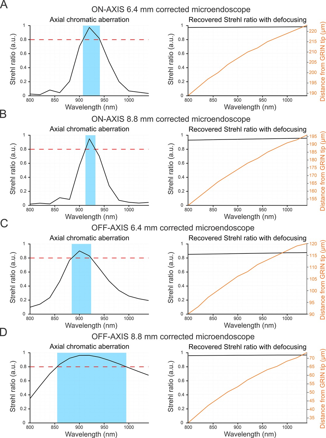
Performance of corrected microendoscopes at different wavelengths.
(A) Left: simulated Strehl ratio on the optical axis as a function of wavelength for the 6.4 mm-long corrected microendoscope. The red dashed line marks the diffraction-limited threshold according to the Maréchal criterion. The area highlighted in light blue indicates the range of wavelengths for which the Strehl ratio is above the diffraction-limited threshold. Right: maximal simulated Strehl ratio obtained on-axis (black line) and corresponding working distance (Distance from GRIN tip, orange line) as a function of wavelength. (B) Same as in (A) for the 8.8 mm-long corrected microendoscope. (C) Same as in (A) for Strehl ratio computed off-axis, considering the largest simulated radial distance from the optical axis used to determine the profile of the corrective lens. In the object plane, this off-axis radial distance is equal to 156 μm. (D) Same as in (C) for the 8.8 mm-long corrected microendoscope and largest simulated radial distance equal to 135 μm.
Figure 1—figure supplement 2
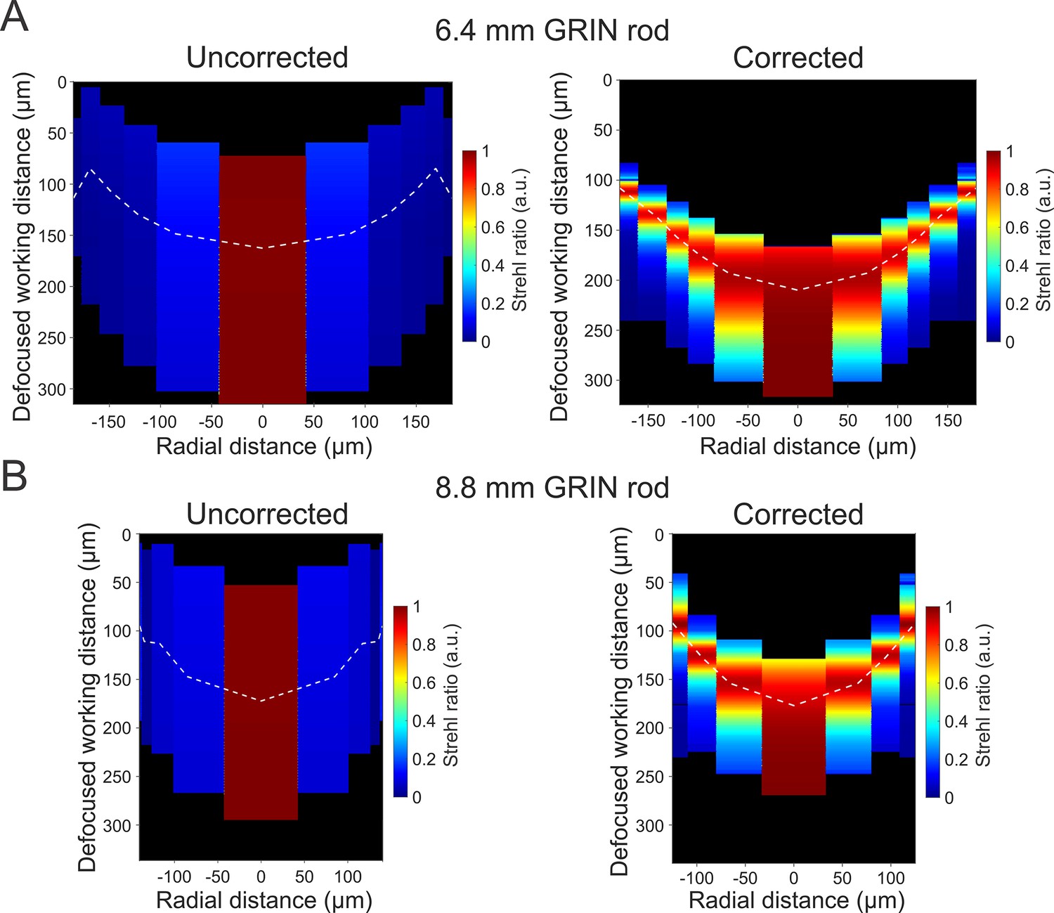
Optical performance in out-of-focus planes.
(A) Pseudocolor map of the Strehl ratio obtained in the object space (x,z projection) at different focal distances (z-axis, Defocused working distance) and as a function of radial distance from the optical axis (corresponding to the zero in the x-axis) computed on the focal plane in the object space for the uncorrected (left) and the corrected (right) 6.4 mm-long microendoscope. For the corrected microendoscope (right), the white dashed line represents the focal plane for which the corrective lens profile was optimized. For the uncorrected microendoscope (left), the white dashed line is the focal plane of the system in the absence of the corrective lens. (B) Same as in (A) for the 8.8 mm-long microendoscope.
Figure 1—figure supplement 3
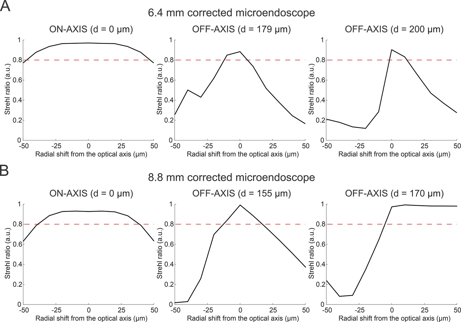
Optical performance of corrected microendoscopes as a function of decentering the corrective lens.
(A) Strehl ratio as a function of radial shift between the corrective lens and the optical axis of the GRIN rod for the 6.4 mm-long corrected microendoscope. Simulation were performed along the optical axis of the GRIN rod (left, on-axis, d=0 µm) and at two marginal radial distances (d, center and right panels; radial distances are computed on the focal plane in the image space, before the GRIN rod). The red dashed line marks the diffraction-limited threshold according to the Maréchal criterion. (B) Same as in (A) for the 8.8 mm-long corrected microendoscope.
Figure 2
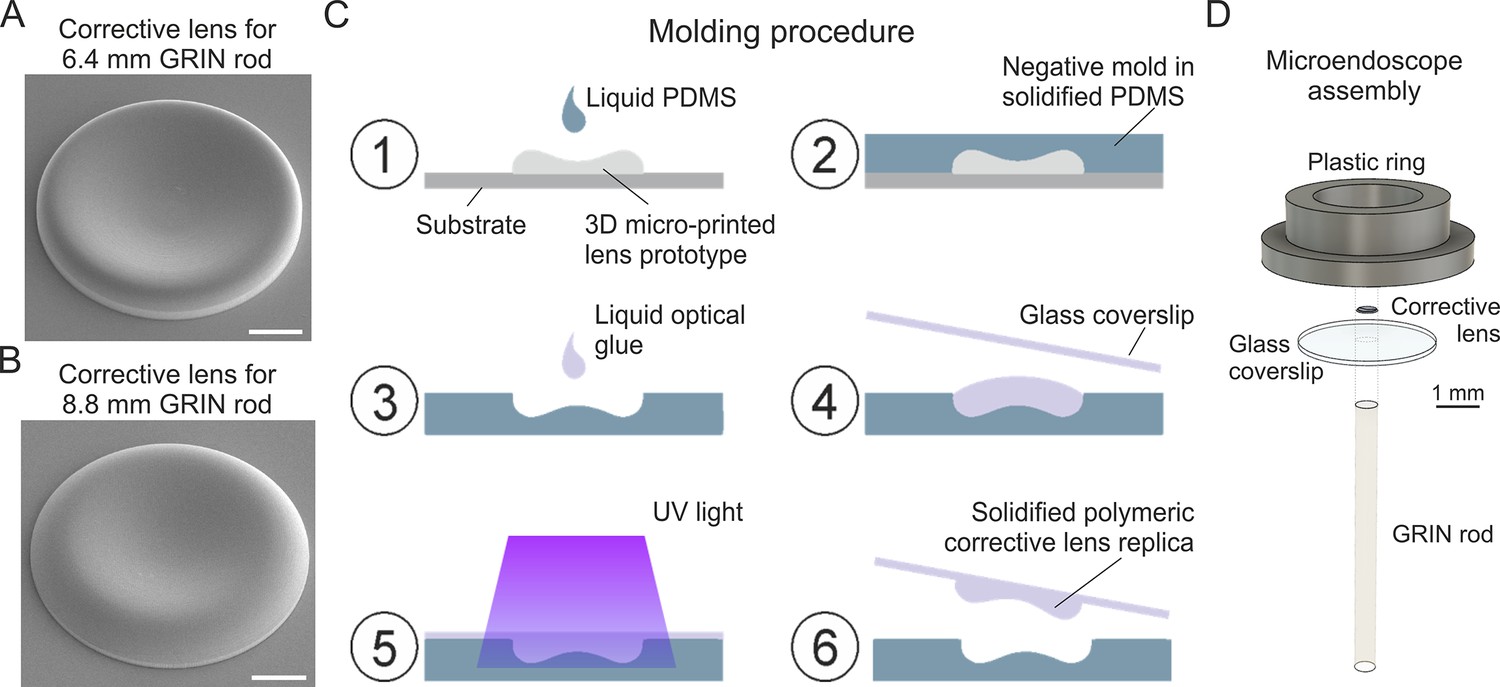
Fabrication of corrective lenses using 3D microprinting and assembly of long microendoscopes.
(A) Scanning electron microscopy image of the 3D microprinted replica of the corrective lens for the 6.4 mm-long corrected microendoscope. Scale bar: 100 µm. (B) Same as (A) for the 8.8 mm-long microendoscope. (C) Molding procedure for the generation of corrective lens replica. Freshly prepared PDMS is casted onto a corrective aspherical lens printed with 2P lithography (1). After 48 hr, the solidified PDMS provides a negative mold for the generation of lens replica (2). A small drop of optical UV-curable glue is deposited onto the mold (3). The mold filled by optical glue is covered with a glass coverslip, which is gently pressed against the mold (4). The optical glue is polymerized with UV light (5). The coverslip with the attached polymeric lens replica is detached from the negative mold (6). Object dimensions are not to scale. (D) Exploded view of the corrected microendoscope assembly.
Figure 3
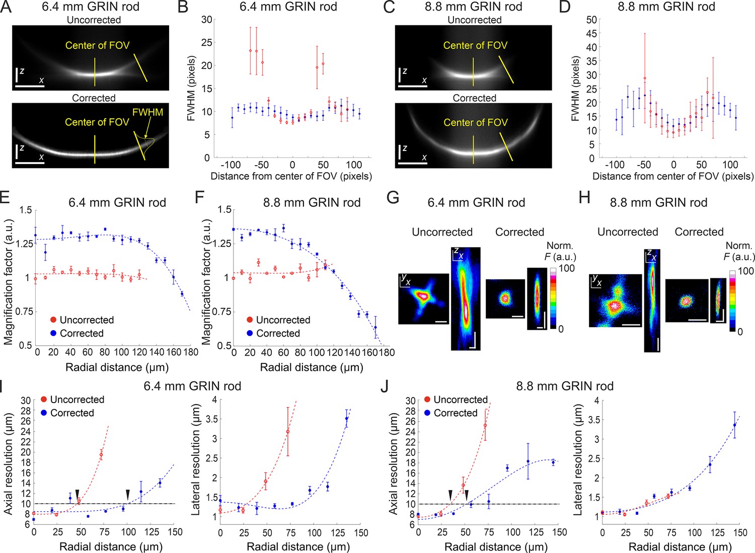
Optical characterization of long corrected microendoscopes shows improved spatial resolution over an enlarged FOV.
(A) Representative x (horizontal), z (vertical) projection of a z-stack of a subresolved fluorescent layer acquired with the uncorrected (top) or corrected (bottom) microendoscope based on the 6.4 mm-long GRIN rod. λexc=920 nm; scale bars: 50 pixels. (B) Thickness (mean values ± s.e.m.) of the layer as a function of the distance from the center of the FOV for uncorrected (red, n=4) or corrected (blue, n=4) microendoscopes. The thickness of the film is measured as the FWHM of the Gaussian fit of the fluorescence intensity along segments orthogonal to the tangential line to the section of the film and located at different distances from the center of the FOV (see yellow labels on the bottom image). (C,D) Same as (A,B) for the microendoscope based on the 8.8 mm-long GRIN rod. (E) The distortion of the FOV in uncorrected and corrected microendoscopes is evaluated using a calibration ruler. The magnification factor is defined as the ratio between the nominal and the real pixel size of the image and shown as a function of the radial distance for uncorrected (red, n=3) or corrected (blue, n=3) microendoscopes. Data are shown as mean values ± s.e.m. Fitting curves are quartic functions f(x)=ax4+bx2+c (see also Supplementary file 3 for details). (F) Same as (E) for the microendoscope based on the 8.8 mm-long GRIN rod. (G–J) The spatial resolution of microendoscopes was measured acquiring z-stacks of subresolved fluorescent beads (bead diameter: 100 nm) located at different radial distances using 2PLSM (λexc=920 nm). (G) Representative x,y and x,z projections of a fluorescent bead located at a radial distance of 75 μm, imaged through an uncorrected (left) or a corrected (right) 6.4 mm-long microendoscope. Horizontal scale bars, 2 μm; vertical scale bars, 5 μm. (H) Same as (G) for the microendoscope based on the 8.8 mm-long GRIN rod. (I) Axial (left) and lateral (right) resolution (i.e. average size of the x,z and x,y projections of imaged beads, respectively) as a function of the radial distance from the center of the FOV for uncorrected (red) and corrected (blue) probes. Each data point represents the mean value ± s.e.m. of n=4–24 beads imaged using at least m=3 different 6.4 mm-long microendoscopes. Fitting curves are quartic functions f(x)=ax4+bx2+c (see Supplementary file 4 for details). The horizontal black dash-dotted line indicates the axial resolution threshold of 10 µm. The black triangles indicate the intersections between the threshold and the curves fitting the data and mark the estimated radius of the effective FOV of the probes. (J) Same as (I) for the microendoscopes based on the 8.8 mm-long GRIN rod.
-
Figure 3—source data 1
Numerical values to reproduce graphs in Figure 3B, D–F,I and J.
- https://cdn.elifesciences.org/articles/101420/elife-101420-fig3-data1-v1.csv
Figure 4 with 1 supplement
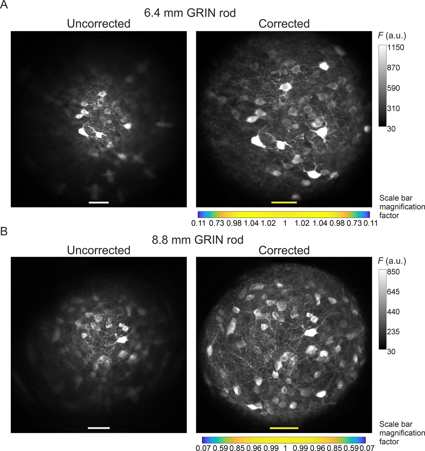
Aberration correction in long GRIN lens-based microendoscopes enables high-resolution imaging of biological structures over enlarged FOVs.
(A) jGCaMP7f-stained neurons in a mouse fixed brain slice were imaged using 2PLSM (λexc=920 nm) through an uncorrected (left) and a corrected (right) microendoscope based on the 6.4 mm-long GRIN rod. Images are maximum fluorescence intensity (F) projections of a z-stack acquired with a 5 μm step size. Number of steps: 32 and 29 for uncorrected and corrected microendoscope, respectively. Scale bars: 50 μm. Left: the scale applies to the entire FOV. Right: the scale bar refers only to the center of the FOV; off-axis scale bar at any radial distance (x and y axes) is locally determined multiplying the length of the drawn scale bar on-axis by the corresponding normalized magnification factor shown in the horizontal color-coded bar placed below the image (see also Figure 3, Supplementary file 3, and Materials and methods for more details). (B) Same results for the microendoscope based on the 8.8 mm-long GRIN rod. Number of steps: 23 and 31 for uncorrected and corrected microendoscope, respectively.
Figure 4—figure supplement 1
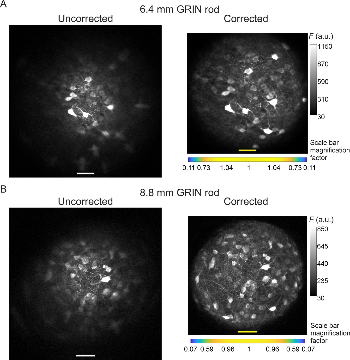
Modified version of Figure 4 with the FOVs of corrected microendoscopes rescaled to match the real pixel size of the FOVs of uncorrected microendoscopes in the center of the image.
See caption of Figure 4. In Figure 4A and B, images acquired with corrected microendoscopes (right images) have a real pixel size in the center of the FOV smaller than the pixel size in the center of the FOVs of uncorrected microendoscopes (left images), due to distortion introduced by corrective lenses (Figure 3E and F). Here, the FOV of corrected microendoscopes (right images) are scaled in order to have the scale bar in the center of the FOV equal to the one of the FOV of uncorrected microendoscopes (left images).
Figure 5
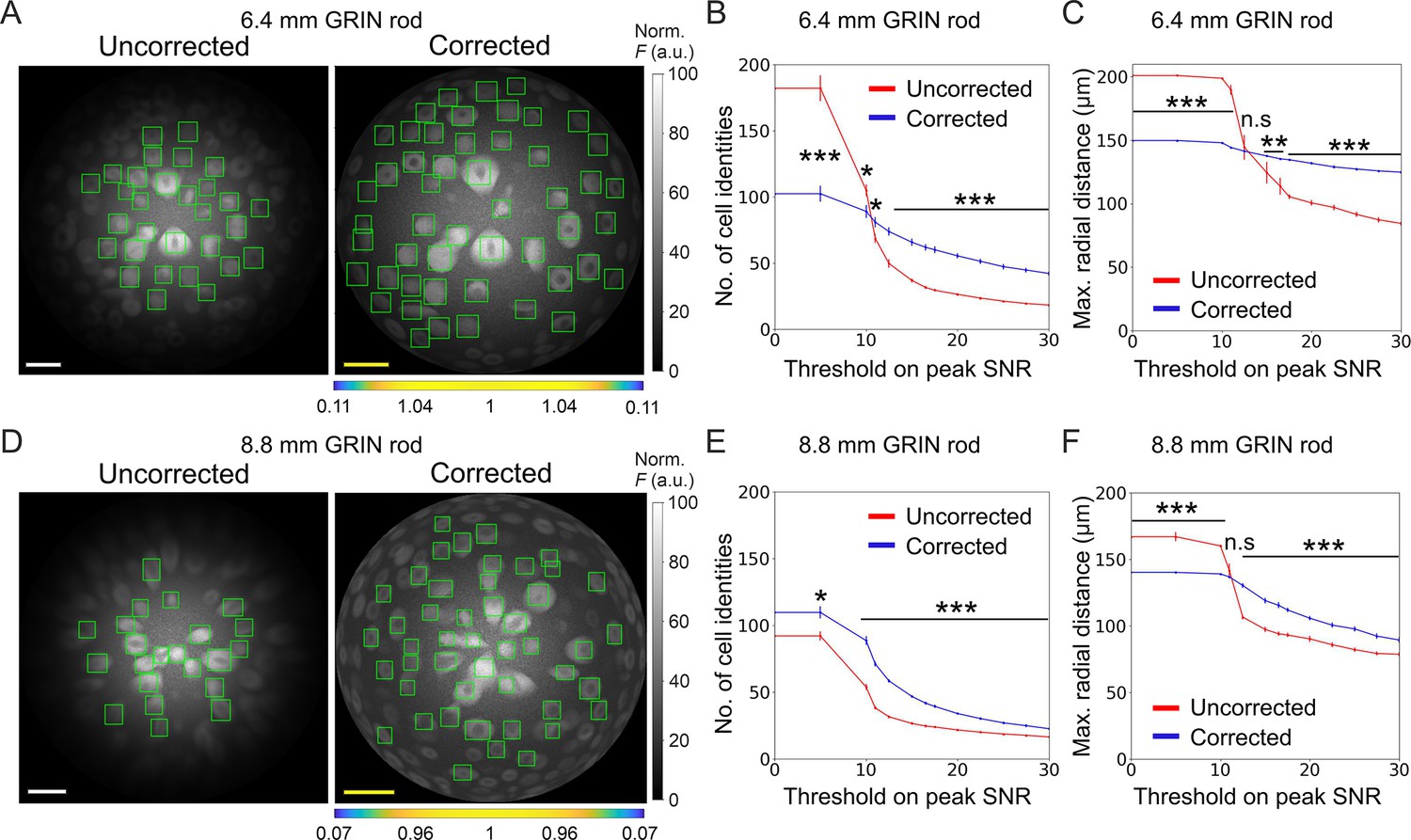
Long corrected microendoscopes sample more homogeneously simulated neuronal activity across the FOV.
(A) Median fluorescence intensity (F) projections of representative synthetic t-series for the uncorrected (left) and the corrected (right) 6.4 mm-long microendoscope. Cell identities were detected using CITE-ON Sità et al., 2022 in n=13 simulated t-series for both the uncorrected and corrected microendoscopes and cellular activity traces were extracted. Green rectangular boxes mark cell identities that have peak SNR of the activity trace higher than a threshold set to peak SNR = 15. Scale bars: 50 μm. Left: the scale applies to the entire FOV. Right: the scale bar refers to the center of the FOV; off-axis scale bar at any radial distance (x and y axes) is locally determined multiplying the length of the drawn scale bar by the corresponding normalized magnification factor shown in the horizontal color-coded bar placed below the image. (B) Number of detected cell identities in simulated FOV as a function of peak SNR threshold imposed on cellular activity traces. Data are mean values ± s.e.m. for both the uncorrected (red) or corrected (blue) case. Statistical significance is assessed with Mann-Whitney U test; *, p<0.05; ***, p<0.001. (C) Maximal distance from the center of the FOV at which a cell is detected as a function of peak SNR threshold. Data are mean values ± s.e.m. for both the uncorrected (red) and corrected (blue) case. Statistical significance is assessed with Mann-Whitney U test; **, p<0.01; ***, p<0.001; n.s., not significant. (D) Same as (A) for the 8.8 mm long microendoscope. (E,F) Same as (B,C) for n=15 simulated t-series for both the uncorrected and corrected 8.8 mm-long microendoscope.
-
Figure 5—source data 1
Numerical values to reproduce graphs in Figure 5B, C, E and F.
- https://cdn.elifesciences.org/articles/101420/elife-101420-fig5-data1-v1.csv
Figure 6 with 2 supplements
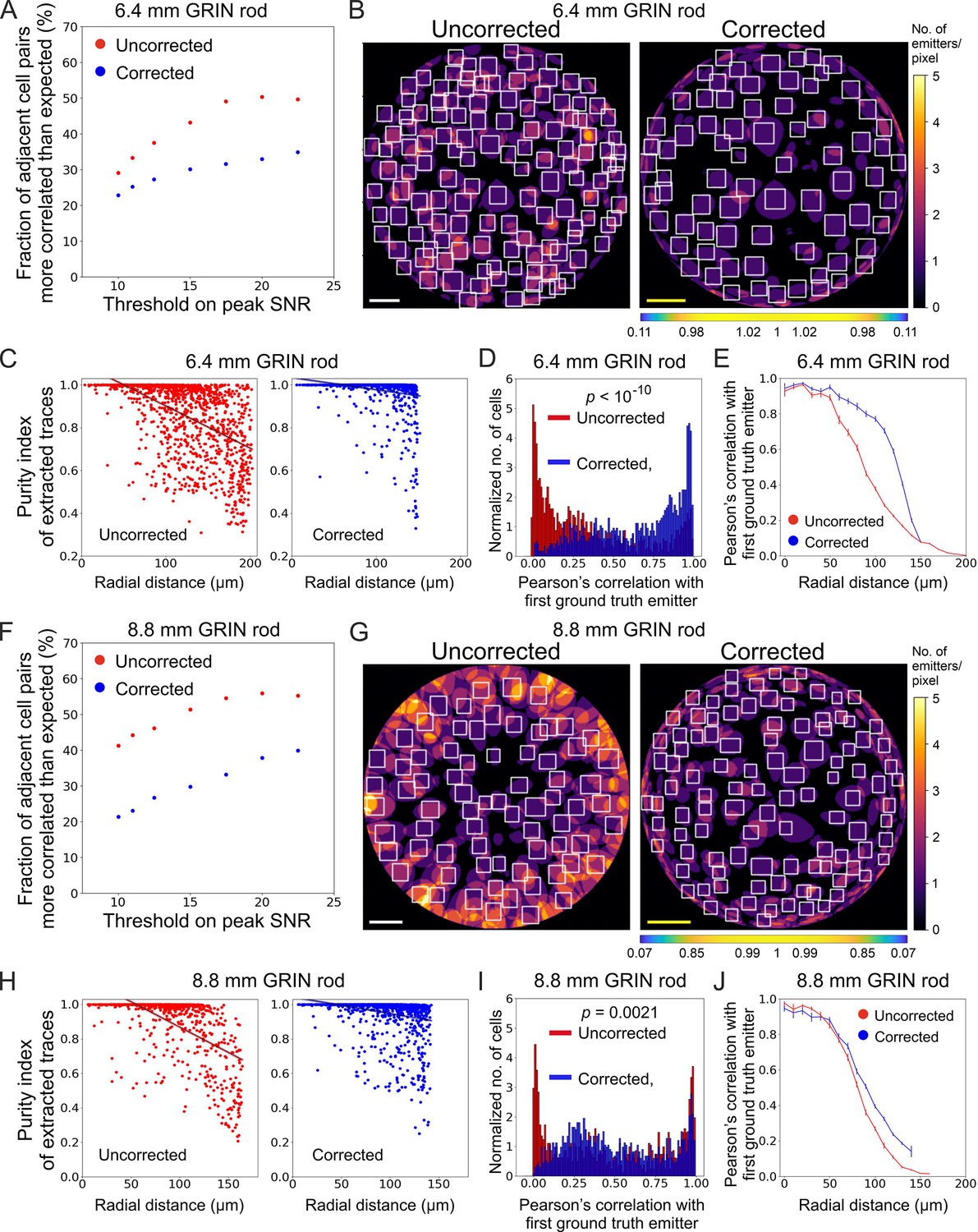
Long corrected microendoscopes enable more precise collection of simulated activity signals from individual cellular sources and decrease cross-contamination between adjacent cells.
(A) Fraction of adjacent cell pairs (distance between detected cell centroids ≤25 µm) that are more correlated that expected (expected pair correlation was estimated as mean Pearson’s correlation between ground truth activity traces of any possible neuronal pairs plus 3 SDs) as a function of the peak SNR threshold imposed on extracted activity traces for n=13 simulated experiments with the 6.4 mm-long uncorrected (red) and corrected (blue) microendoscope. (B) 2D projection of the intersection between the 3D FOV and the 3D ground truth distribution of light sources for a representative uncorrected (left) and corrected (right) synthetic t-series obtained with a 6.4 mm-long microendoscope. The color scale shows the number of overlapping sources that are projected on the same pixel. White boxes mark cell identities detected using CITE-ON (Sità et al., 2022) without any threshold on the peak SNR of activity traces. Scale bars: 50 μm. Left: the scale applies to the entire FOV. Right: the scale bar refers to the center of the FOV; off-axis scale bar at any radial distance (x and y axes) is locally determined multiplying the length of the scale bar by the corresponding normalized magnification factor shown in the horizontal color-coded bar placed below the image. (C) Purity index of extracted traces with peak SNR >10 was estimated using a GLM of ground truth source contributions and plotted as a function of the radial distance of cell identities from the center of the FOV for n=13 simulated experiments with the 6.4 mm-long uncorrected (red) and corrected (blue) microendoscope. Black lines represent the linear regression of data ± 95% confidence intervals (shaded colored areas). Slopes ± s.e.: uncorrected, (–0.0020±0.0002) μm–1; corrected, (–0.0006±0.0001) μm–1. Uncorrected, n=1365; corrected, n=1,156. Statistical comparison of slopes, p<10–10, permutation test. Linear regression was repeated using the same range of radial distances for the uncorrected and corrected case, with the maximum value on the x-axis corresponding to the minimum value between the two maximum radial distances obtained in the uncorrected and corrected case (maximum radial distance: 151.6 µm); slopes ± s.e.: uncorrected, (–0.0015±0.0002) µm–1; corrected, (–0.0006±0.0001) μm–1. Uncorrected, n=991; corrected, n=1,156. Statistical comparison of slopes, p<10–10, permutation test. (D) Distribution of the Pearson’s correlation value of extracted activity traces with the first (most correlated) ground truth source for n=13 simulated experiments with the 6.4 mm-long uncorrected (red) and corrected (blue) microendoscope. Median values: uncorrected, 0.25; corrected, 0.73; the p is computed using the Mann-Whitney U test. (E) Pearson’s correlation ± s.e.m. of extracted activity traces with the first (most correlated) ground truth emitter as a function of the radial distance for n=13 simulated experiments with the 6.4 mm-long uncorrected (red) and corrected (blue) microendoscope. (F–J) Same as (A–E) for n=15 simulated experiments with the 8.8 mm-long uncorrected and corrected microendoscope. (H) Slopes ± s.e.: uncorrected, (–0.0031±0.0003) μm–1; corrected, (–0.0010±0.0002) μm–1. Uncorrected, n=808; corrected, n=1,328. Statistical comparison of slopes, p<10–10, permutation test. Linear regression using the same range of radial distances for the uncorrected and corrected case (maximum radial distance: 142.1 μm), slopes ± s.e.: uncorrected, (–0.0014±0.0003) μm–1; corrected, (–0.0010±0.0002) µm–1. Uncorrected, n=718; corrected, n=1328. Statistical comparison of slopes, p=0.0082, permutation test. (I) Median values: uncorrected, 0.43; corrected, 0.46; the p is computed using the Mann-Whitney U test.
-
Figure 6—source data 1
Numerical values to reproduce graphs in Figure 6A and C–E.
- https://cdn.elifesciences.org/articles/101420/elife-101420-fig6-data1-v1.csv
-
Figure 6—source data 2
Numerical values to reproduce graphs in Figure 6F and H–J.
- https://cdn.elifesciences.org/articles/101420/elife-101420-fig6-data2-v1.csv
Figure 6—figure supplement 1
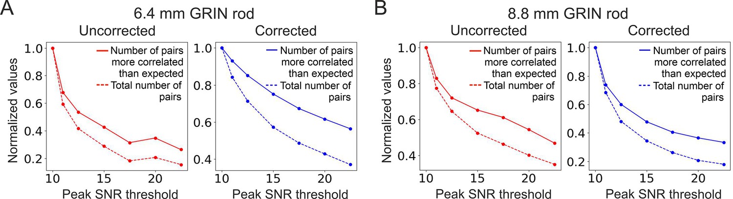
The total number of detected adjacent cell pairs decreases faster with peak SNR threshold than the number of adjacent cell pairs more correlated than expected does.
(A) Number of adjacent cell pairs more correlated than expected (solid lines) and total number of detected adjacent cell pairs (dashed lines) as a function of the peak SNR threshold for the uncorrected (red, left) and the corrected (blue, right) 6.4 mm-long microendoscope (see also Figure 6A). Values are normalized to their value at peak SNR threshold = 10. (B) Same as (A) for the 8.8 mm-long microendoscope (see also Figure 6F).
Figure 6—figure supplement 2
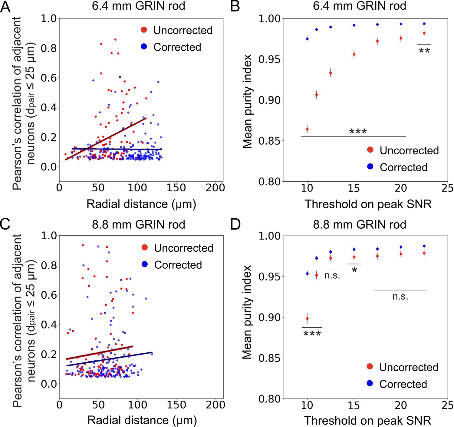
Aberration correction enables more accurate measurement of population activity.
(A) Pearson’s correlation of adjacent cell pairs as a function of the radial distance from the center of the FOV in simulated calcium data. Pairs of cells were defined as adjacent if the distance between detected cell centroids dpair was ≤25 µm. Pearson’s correlation is displayed only for cell pairs which are more correlated than expected (expected pair correlation was estimated as mean Pearson’s correlation between ground truth activity traces of any possible neuronal pairs plus 3 SDs, see Supplementary file 5). Data are displayed only for cells with peak SNR >15 from n=13 simulated experiments with the 6.4 mm-long uncorrected (red) and corrected (blue) microendoscope. Black lines represent the linear regression of data ±95% confidence intervals (shaded colored areas). Slopes ±s.e.: uncorrected, (0.003±0.002) μm–1, significantly different from zero, p=0.00080, permutation test; corrected, (–0.00003±0.00060) μm–1, not significantly different from zero, p=0.88, permutation test. Uncorrected, n=102; corrected, n=172. Statistical comparison of slopes, p<10–10, permutation test. (B) Mean purity index (see Materials and methods for definition)± s.e.m. of extracted traces as a function of the peak SNR threshold for n=13 simulated experiments with the 6.4 mm-long uncorrected (red) and corrected (blue) microendoscope. Statistical differences of the means are assessed with the permutation test; **, p<0.01; ***, p<0.001. (C) Same as (A) for n=15 simulated experiments with the 8.8 mm-long uncorrected and corrected microendoscope. Slopes ±s.e.: uncorrected, (0.001±0.002) μm–1, not significantly different from zero, p=0.41, permutation test; corrected, (0.0008±0.0013) μm–1, not significantly different from zero, p=0.20, permutation test. Uncorrected, n=96; corrected, n=152. Statistical comparison of slopes, p=0.86, permutation test. (D) Same as (B) for n=15 simulated experiments with the 8.8 mm-long uncorrected and corrected microendoscope. *, p<0.05; ***, p<0.001; n.s., not significant.
Figure 7
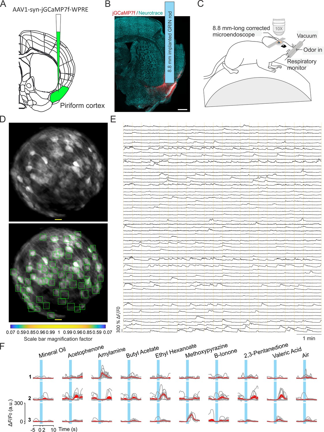
Enlarged FOV population imaging of ventral regions of the brain with long corrected microendoscopes in awake mice.
(A) Schematic showing injection of the viral solution in the mouse piriform cortex. (B) Representative section of fixed brain tissue showing the position of the GRIN lens implant. jGCaMP7f fluorescence is shown in red. NeuroTrace (Neurotrace) Nissl staining is shown in cyan. (C) Schematic showing the experimental preparation for 2P corrected microendoscope imaging in awake mice. (D) Top and bottom: example of FOV with excitatory neurons expressing the calcium sensor jGCaMP7f, obtained using the 8.8 mm-long corrected microendoscope in the mouse piriform cortex. The bottom image shows the rectangular boxes (green) indicating the position of detected neurons generated by CITE-ON (see Materials and methods, Sità et al., 2022). On-axis scale bar: 20 µm; for off-axis scale bar, refer to the magnification factor bar below the image (see Materials and methods). (E) Representative jGCaMP7f activity traces extracted from the recording shown in (D) through 8-min-long continuous 2P imaging recordings (=920 nm) in an awake head-fixed mouse. Vertical dashed orange lines mark the onset and the end of the 22-s-long trials in which the imaging session was divided. (F) Examples of neuronal responses to different olfactory stimuli for three representative cells. For each odor (top labels), gray lines represent calcium responses recorded in single trials and the red line represent the average response. Light blue areas indicate the time interval of stimulus presentation.
Figure 8
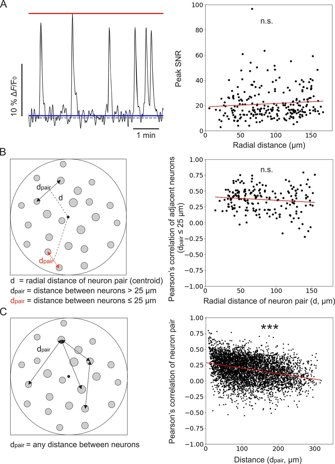
Unbiased population imaging in the piriform cortex of awake mice using long corrected microendoscopes.
(A) Left: schematic representation of trace parameters used to compute peak SNR. The red solid line marks the maximum value of the trace, the blue line indicates the SD of intensity values below the 25th percentile of the intensity distribution of the entire trace (see Materials and methods), and the dashed grey line marks the origin of the y-axis (ΔF/F0=0). Right: peak SNR of calcium traces extracted from individual cells as a function of radial distance of the cell (n=240 neurons from m=6 FOVs). The red line is the linear regression of data points: intercept ±s.e.=19 ± 2; slope ±s.e. = (0.03±0.02) μm–1. The slope is not significantly different from zero, p=0.18, permutation test. (B) Left: schematic representation showing pairs of neurons and distance definitions for the Pearson’s correlation analysis shown on the right (in red, distance between ‘adjacent neurons’ dpair ≤25 µm). Right: Pearson’s correlation of calcium traces from ‘adjacent neurons’ as a function of radial distance of the pair centroid from the center of the FOV (n=195 adjacent neuron pairs from m=6 FOVs). The red line represents the linear regression of data points: intercept ±s.e.=0.41 ± 0.03; slope ±s.e. = (–0.0006±0.0004) μm–1. The slope is not significantly different from zero, p=0.089, Wald test. (C) Left: schematic representation of neuron pairs used for the analysis on the right (any possible dpair). Right: Pearson’s correlation of calcium traces from pairs of neurons as a function of the distance between them (n=4767 pairs from m=6 FOVs). The red line is the linear regression of data points: intercept ±s.e.=0.288 ± 0.005; slope ±s.e. = (–87±4) ∙ 10–5 μm–1. The slope is significantly different from zero, p=2 ∙ 10–5, permutation test.
-
Figure 8—source data 1
Numerical values to reproduce graphs in Figure 8A–C, right panels.
- https://cdn.elifesciences.org/articles/101420/elife-101420-fig8-data1-v1.csv
Tables
Table 1
Experimental measurement of enlarged effective FOV in long corrected microendoscopes.
The values of the effective FOV radius for uncorrected and corrected microendoscopes were estimated from the intersection between the arbitrary threshold of 10 µm on the axial resolution and the quartic function fitting the experimental data of Figure 3I and J.
| Microendoscope type | Effective FOV radius (µm) | Fold increase inFOV radius | Fold increase inFOV area |
|---|---|---|---|
| 6.4 mm-long GRIN rod | Uncorrected: 46 Corrected: 100 | 2.17 | 4.7 |
| 8.8 mm-long GRIN rod | Uncorrected: 34 Corrected: 52 | 1.53 | 2.3 |
Table 2
Characteristics of commercially available (Commercial) and customized (Custom) GRIN rods used for simulation and fabrication of aberration corrected microendoscopes.
All GRIN rods were obtained from GRINTECH GmbH, Jena, Germany.
| 6.4 mm-long GRIN rod | 8.8 mm-long GRIN rod | |||
|---|---|---|---|---|
| Commercial | Custom | Commercial | Custom | |
| Catalogue # | NEM-050-25-10-860-S-1.5p | NEM-050-25-15-860-S-1.5p | NEM-050-25-10-860-S-2.0p | NEM-050-23-15-860-S-2.0p |
| Diameter (µm) | 500 | 500 | 500 | 500 |
| Length (mm) | 6.52 | 6.4 | 8.85 | 8.8 |
| Working distance (µm) | Image side: 100 Object side: 250 | Image side: 150 Object side: 250 | Image side: 100 Object side: 250 | Image side: 150 Object side: 230 |
Key resources table
| Reagent type (species) or resource | Designation | Source or reference | Identifiers | Additional information |
|---|---|---|---|---|
| Strain, strain background (Mus musculus; males, females) | C57BL/6 J | Jackson Laboratory | Strain #: 000664; RRID:IMSR_JAX:000664 | |
| Genetic reagent (Mus musculus; males, females) | Ai14 | Jackson Laboratory | Strain #: 007914; RRID:IMSR_JAX:007914 | |
| Recombinant DNA reagent | pGP-AAV-syn-jGCaMP8f-WPRE | Addgene, Zhang et al., 2023 | Catalog #: 162376-AAV1 | Dilution: 1/3 in PBS |
| Recombinant DNA reagent | AAV1-syn-jGCaMP7f-WPRE | Addgene Dana et al., 2019 | Catalog #: 104488-AAV1 | Dilution: 1/3 in PBS |
| Chemical compound, drug | Photoresin | Nanoscribe | Resin: IP-S | |
| Chemical compound, drug | UV-curable glue, NOA63 | Norland Products | Product: NOA63 | |
| Chemical compound, drug | Poly-l-lysine | Merck | Product No.: P2636 | Dilution: 0.1 mg/mL in water |
| Commercial assay or kit | PDMS, Sylgard 184 Silicone Elastomer Kit | Dow | Material No.: 4019862 | |
| Commercial assay or kit | Metabond adhesive cement | Parkell | SKU: S396 | |
| Commercial assay or kit | Dental cement, Pi-ku-plast HP 36 Precision Pattern Resin | XPdent | SKU #: 54000210 SKU #: 54000215 | |
| Commercial assay or kit | Kwik-Sil silicone elastomer | World Precision Instruments | Code: KWIK-CAST | |
| Software, algorithm | OpticStudio 15 | Zemax (Ansys) | https://www.ansys.com/products/optics/ansys-zemax-opticstudio | |
| Software, algorithm | CAD | SolidWorks | https://www.solidworks.com/product/solidworks-3d-cad | |
| Software, algorithm | Imagej/Fiji | NIH (open source) | RRID:SCR_002285 | https://fiji.sc/ |
| Software, algorithm | Matlab R2022b, Matlab | MathWorks | RRID:SCR_001622 | https://it.mathworks.com/products/new_products/release2022b.html |
| Software, algorithm | CITE-ON | Sità et al., 2022; Sità et al., 2021 | Optical Approaches to Brain Function Laboratory, Istituto Italiano di Tecnologia; https://gitlab.iit.it/fellin-public/cite-on | |
| Software, algorithm | Python 3.7, Python | Python Software Foundation | RRID:SCR_008394 | https://www.python.org/downloads/release/python-370/ |
| Software, algorithm | Software for generation of artificial t-series | This paper; Antonini et al., 2020 | Optical Approaches to Brain Function Laboratory, Istituto Italiano di Tecnologia. See Data and software availability section in this paper and in Antonini et al., 2020 | |
| Other | 6.4 mm-long GRIN rod | GRINTECH | Product code: NEM-050-25-10-860-S-1.5p | Customized product |
| Other | 8.8 mm-long GRIN rod | GRINTECH | Product code: NEM-050-25-10-860-S-2.0p | Customized product |
| Other | 3D microprinter | Nanoscribe | Photonic Professional GT2+ | |
| Other | Chameleon Ultra II laser source | Coherent | Chameleon Ultra II | |
| Other | Chameleon Discovery laser source | Coherent | Chameleon Discovery | |
| Other | Investigator scan head | Bruker Corporation | Ultima Investigator | |
| Other | Ultima IV scan head | Bruker Corporation | Prairie Technologies Ultima IV | |
| Other | 20 x dry objective, objective | Zeiss | EC Epiplan-Neofluar 20 x/0,50 Ph2 M27 | For optical characterizations |
| Other | 10 X Plan Apochromat Lambda objective, objective | Nikon | Plan Apochromat Lambda D 10 x/0.45 | For in vivo imaging |
| Other | 16-channel olfactometer | AutoMate Scientific | Customized product | |
| Other | Photoionization detector | Aurora Scientific | Product: 200B: miniPID Fast Response Olfaction Sensor | |
| Other | Calibration ruler, 4-dot calibration slide | Motic | Product code: 1101002300142 | |
| Other | Fluorescent beads, FluoSpheres Carboxylate-Modified Microspheres | Thermo Fisher | Catalog No.: F8803 | Diameter: 100 nm |
| Other | Teensy 3.6 | PJRC | Product: Teensy 3.6 Development Board |
Table 3
Working distances of uncorrected and corrected microendoscopes based on long GRIN lenses obtained with ray-trace simulations shown in Figure 1.
| Microendoscope based on 6.4 mm-long GRIN rod | Microendoscope based on 8.8 mm-long GRIN rod | |||
|---|---|---|---|---|
| Uncorrected | Corrected | Uncorrected | Corrected | |
| Working distances (μm) | Image side: 150 Object side: 215 | Image side: 150 Object side: 210 | Image side: 145 Object side: 228 | Image side: 143 Object side: 178 |
Additional files
-
Supplementary file 1
Parameters of the polynomial function describing the aspherical surface of simulated corrective lenses.
Parameters of Equation 1 (see Materials and Methods) for the simulated corrective lens designed to be applied to the GRIN rods of length 6.4 mm (top row) and 8.8 mm (bottom row).
- https://cdn.elifesciences.org/articles/101420/elife-101420-supp1-v1.docx
-
Supplementary file 2
Spatial resolution of simulated uncorrected and corrected microendoscopes.
Axial and lateral resolution of simulated microendoscopes were evaluated measuring the dimensions of simulated 2P PSF for each probe at different radial distances. x,z (Axial) and x,y (Lateral) intensity profiles of simulated PSFs were fitted with Gaussian curves and their FWHM was used to define the resolution, as done for experimental PSFs (see Materials and Methods).
- https://cdn.elifesciences.org/articles/101420/elife-101420-supp2-v1.docx
-
Supplementary file 3
Parameters used for the computation of the local pixel size and for distance calibration of images acquired with microendoscopes.
Coefficients of the quartic functions fitting the measurements performed on images acquired on the calibration ruler for uncorrected and corrected microendoscopes based on the 6.4 mm-long GRIN rod (left) and the 8.8 mm-long GRIN rod (right). The numbers in parenthesis indicate the 95% lower and upper confidence bounds (see Figure 3E and F). R-square values are indicated for each fit.
- https://cdn.elifesciences.org/articles/101420/elife-101420-supp3-v1.docx
-
Supplementary file 4
Fitting parameters for PSF measurements of uncorrected and corrected microendoscopes.
Coefficients of quartic functions fitting experimental PSF data (axial, top; lateral, bottom) are presented for uncorrected and corrected microendoscopes based on the 6.4 mm-long GRIN rod (left) and the 8.8 mm-long GRIN rod length (right). Parentheses indicate the 95% lower and upper confidence bounds (see Figure 3I and J). R-square values are indicated for each fit.
- https://cdn.elifesciences.org/articles/101420/elife-101420-supp4-v1.docx
-
Supplementary file 5
Expected Pearson’s correlation of cell pair in synthetic calcium data.
Numerical values used to estimate the expected correlation between cell pairs in synthetic calcium t-series are indicated for each microendoscope type. The table displays the mean and SD of Pearson’s correlation between the activity traces of any possible ground truth source neuron pair obtained from n simulated FOVs and the expected cell pair correlation (mean Pearson’s correlation plus three SDs). These parameters were used for the analysis in Figure 6A and F and in Figure 6—figure supplement 2A and C.
- https://cdn.elifesciences.org/articles/101420/elife-101420-supp5-v1.docx
-
Supplementary file 6
Linear regression analysis for pairwise correlation of adjacent neurons as a function of the radial distance of pair centroid for in vivo 2P imaging data.
The values of the slope of the linear fits are indicated ± s.e. for adjacent neurons with maximum centroid distance equal to 25 µm (top) or 30 µm (bottom). Results obtained with jGCaMP8f, jGCaMP7f, and with the merged dataset including both jGCaMP8f and jGCaMP7f are displayed. The number n of adjacent neuron pairs, the p value of the indicated statistical test for the normality of residuals, and the p value of the Wald test on the null hypothesis of slope = 0 are indicated for each condition.
- https://cdn.elifesciences.org/articles/101420/elife-101420-supp6-v1.docx
-
MDAR checklist
- https://cdn.elifesciences.org/articles/101420/elife-101420-mdarchecklist1-v1.docx
Download links
A two-part list of links to download the article, or parts of the article, in various formats.
Downloads (link to download the article as PDF)
Open citations (links to open the citations from this article in various online reference manager services)
Cite this article (links to download the citations from this article in formats compatible with various reference manager tools)
Aberration correction in long GRIN lens-based microendoscopes for extended field-of-view two-photon imaging in deep brain regions
eLife 13:RP101420.
https://doi.org/10.7554/eLife.101420.4


