Research Article

Neuroscience

A general framework for characterizing optimal communication in brain networks

MRC Cognition and Brain Sciences Unit, University of Cambridge, United Kingdom
Institute of Computational Neuroscience, University Medical Center Eppendorf-Hamburg, Hamburg University, Hamburg Center of Neuroscience, Germany
Department of Psychological and Brain Sciences, Indiana University, United States
Department of Psychology, Max Planck Institute for Human Cognitive and Brain Sciences, Germany
International Max Planck Research School on Cognitive Neuroimaging, Spain
Center for Brain and Cognition, Pompeu Fabra University, Spain
Department of Information and Communication Technologies, Pompeu Fabra University, Spain
McConnell Brain Imaging Centre, Montréal Neurological Institute, McGill University, Canada
Department of Health Sciences, Boston University, United States

Apr 17, 2025

https://doi.org/10.7554/eLife.101780.3

Open access
Copyright information

Figures
Tables
Additional files

10 figures, 2 tables and 1 additional file

Figures

Figure 1

Download asset Open asset

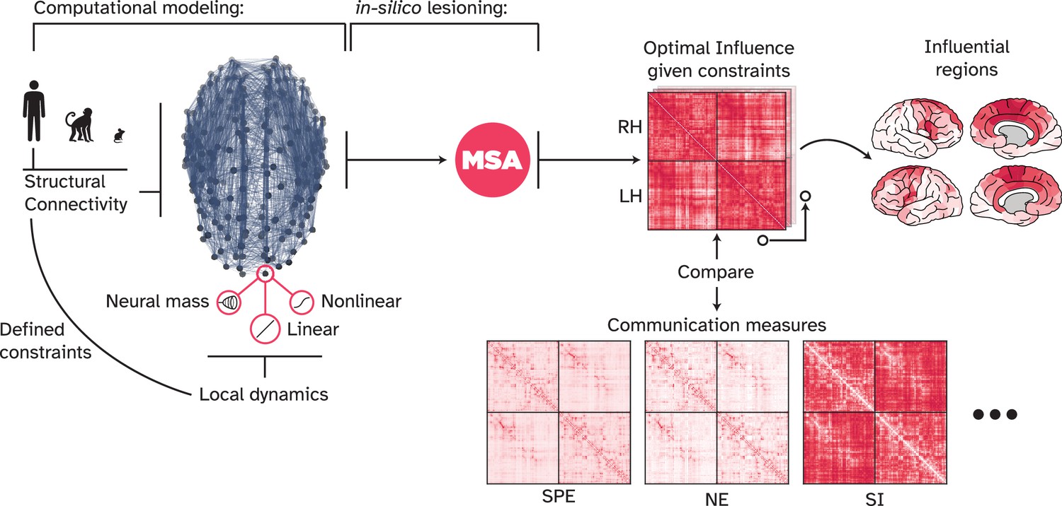
Overview of the present work.

We used the human connectome and a linear model of local node dynamics as the main network model. However, other computational models can be used, building upon different assumptions of local dynamics and other network architectures. Here, we explored Macaque and mouse connectomes, as well as nonlinear models including a neural mass model of local dynamics. These two families of variables, network structure and local dynamics, define our ‘game constraints,’ since they dictate how information flows in the network and how nodes respond to incoming signals. For every game, i.e., a computational model such as a linear model of dynamics on the human connectome, the multi-perturbation Shapley value analysis (MSA) approach (Figure 2) uncovered the ‘optimal influence’ landscape of the network. This landscape describes a game-theoretical equilibrium point at which nodes cannot unilaterally increase their influence on each other any further. We compared the optimal influence profile of nodes at this point with various communication models and analyzed the most influential nodes in such a signal propagation regime. SPE: Shortest path efficiency, NE: Navigation efficiency, SI: Search information.

Figure 2 with 1 supplement

Download asset Open asset

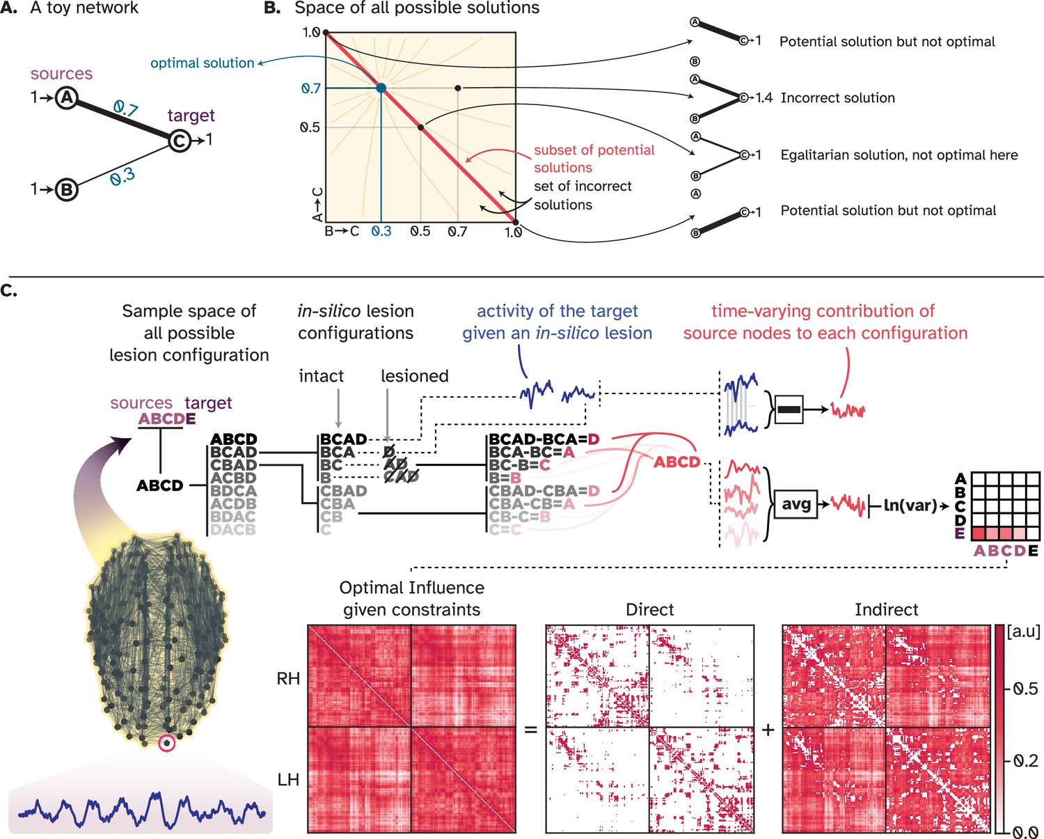
Visual summary of the multi-perturbation Shapley value analysis (MSA) approach.

(A) A simple toy network with two sources and one target, in which the sources have different amounts of influence on the target. (B) For this toy network, the space of all possible ways in which the activity of the target node can be decomposed into contributions from source nodes has two dimensions. There exists a subset of potential solutions where the activity of the target node is correctly decomposed, but the decomposition is not optimal. There exists one equilibrium point where the decomposition is correct and optimal. (C) For every game, that is, the simulation of a whole-brain computational model, MSA performs extensive multi-site lesioning analysis to uncover the influence of every node on every other node. For every target node, MSA lesions combinations of source nodes, track how the activity of the target node changes given each perturbation and, for all source nodes, computes the difference between two scenarios: one with the source node included in the lesion-set, and the other where the source node is not lesioned. The difference between these two cases defines the contribution of the source to that specific coalition/combination of sources. Averaged over all contributions, the time-varying contribution of each source is then inferred. Iterating over all nodes results in the ‘optimal influence’ landscape that can be decomposed into two components: Direct influences, where nodes influence their connected neighbors, and indirect influences, where nodes influence distant unconnected nodes.

Figure 2—figure supplement 1

Download asset Open asset

Comparing the optimal influence matrices from 1000 and 10,000 lesion samples per source node.

Figure 3

Download asset Open asset

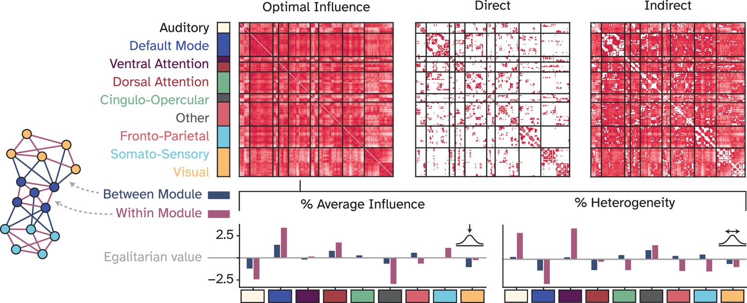
Large-scale network organization of the optimal influence landscape.

Optimal influences were reorganized according to nine large-scale functional network modules and characterized by two metrics: 1. Average influence, which captures the normalized total influence of a given module within itself and to other modules. 2. Heterogeneity of influences, accounting for the normalized variation of influences within a functional module and to other modules. The egalitarian value represents a naive strategy for assigning contributions in which all players are assumed to contribute equally, i.e., by equal division of the total influence among all nine functional modules. The bars represent how much each module deviates positively or negatively from the egalitarian assumption.

Figure 4 with 1 supplement

Download asset Open asset

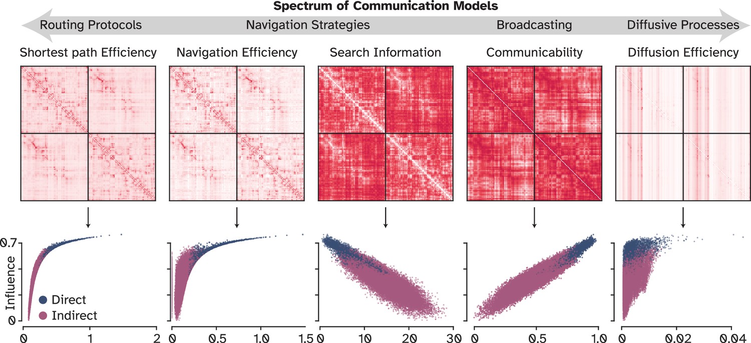
Comparison of optimal influences with other putative communication measures.

Pairwise Pearson’s correlation between each communication measure and optimal influences, to characterize the alignment with existing communication models. Communicability (r=0.94) and Search Information (r=−0.83) had the best alignment in this univariate setting.

Figure 4—figure supplement 1

Download asset Open asset

Comparing optimal influence with functional connectivity.

Figure 5 with 2 supplements

Download asset Open asset

Strategies to alleviate the underestimated influence of long-range pathways.

(A) Difference between adjacency matrices of tunable models and OI that indicates where these models underestimate (red) and overestimate (blue) the influence of nodes on each other. (B) SAR obtains a correlation coefficient of r=0.99 by increasing the depth by which signals can travel, however, the plot on the bottom shows that a wide range of values from 0.2 to 0.7 can be chosen with a small degradation of fit. SAR: Spatial Auto-Regressive model, CO: Communicability, OI: Optimal Influence.

Figure 5—figure supplement 1

Download asset Open asset

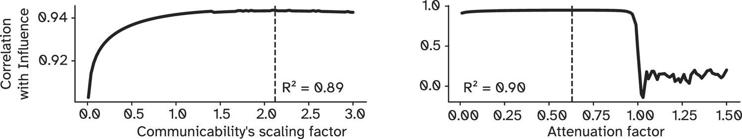
Fitting curve of the scaled communicability (left) and the linear attenuation model (right) to the optimal influence matrix of the human connectome.

Figure 5—figure supplement 2

Download asset Open asset

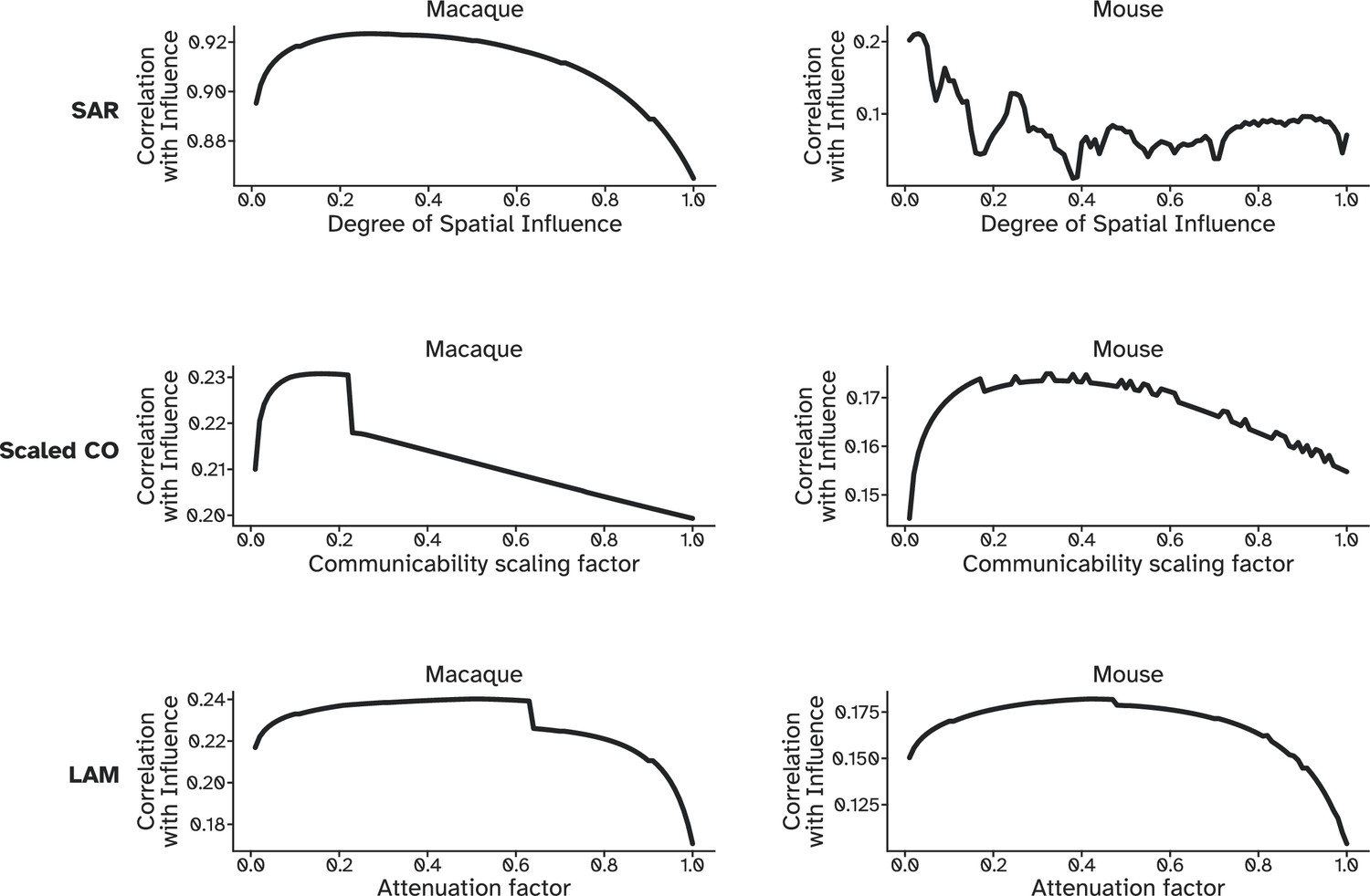
Fitting curves of the spatial autoregressive model (top), scaled communicability (middle) and the linear attenuation model (bottom) to the optimal influence matrix of macaque (left) and mouse (right) connectomes.

Figure 6 with 1 supplement

Download asset Open asset

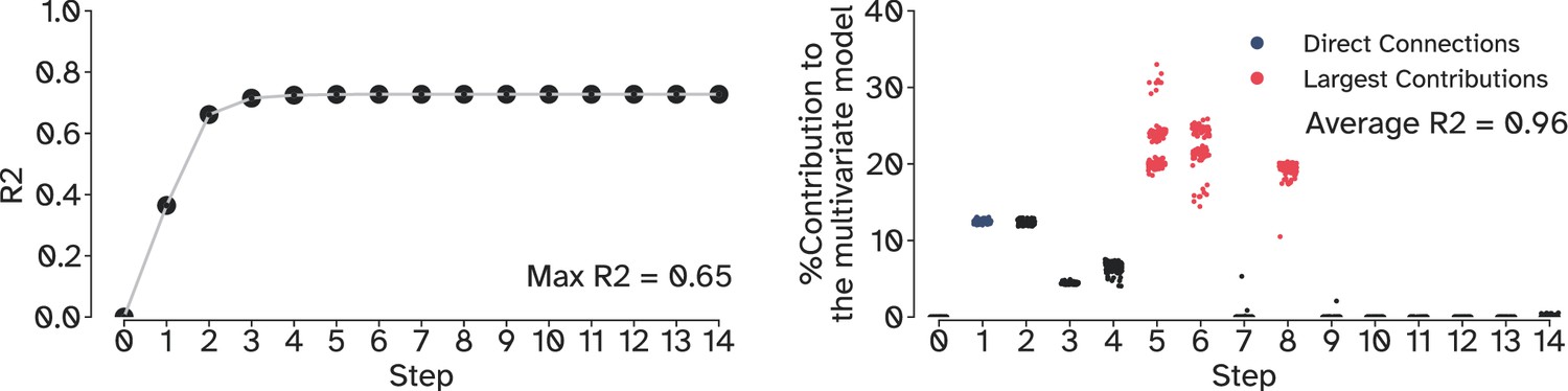
Uni-and-multivariate models of OI.

(A) Predictive power of a linear regression model trained on walks up to 15 broadcasting steps. (B) A regularized multivariate model trained on all steps shows a small set of steps to be sufficient to explain 96% of OI on average. Each dot represents one cross-validation trial (N=100). (C) Sets of regularized multivariate models were trained on network features at each degree of spatial influence for spatial autoregressive model (SAR) and linear attenuation model (LAM) to capture the impact of this parameter on the performance of the statistical model. The dashed line on the left shows a scenario when the degree of spatial influence is zero, effectively rendering SAR an identity matrix. The second dashed line indicates where the model performed the best, explaining 99% OI. (D) Bars represent the contribution of each feature to the model, averaged over degrees of influence. Error bars indicate the 95% confidence interval. OI: Optimal influence.

Figure 6—figure supplement 1

Download asset Open asset

The amount of which univariate and multivariate models can predict optimal influence from summing individual walks, discounted exponentially (as with communicability).

Figure 7 with 1 supplement

Download asset Open asset

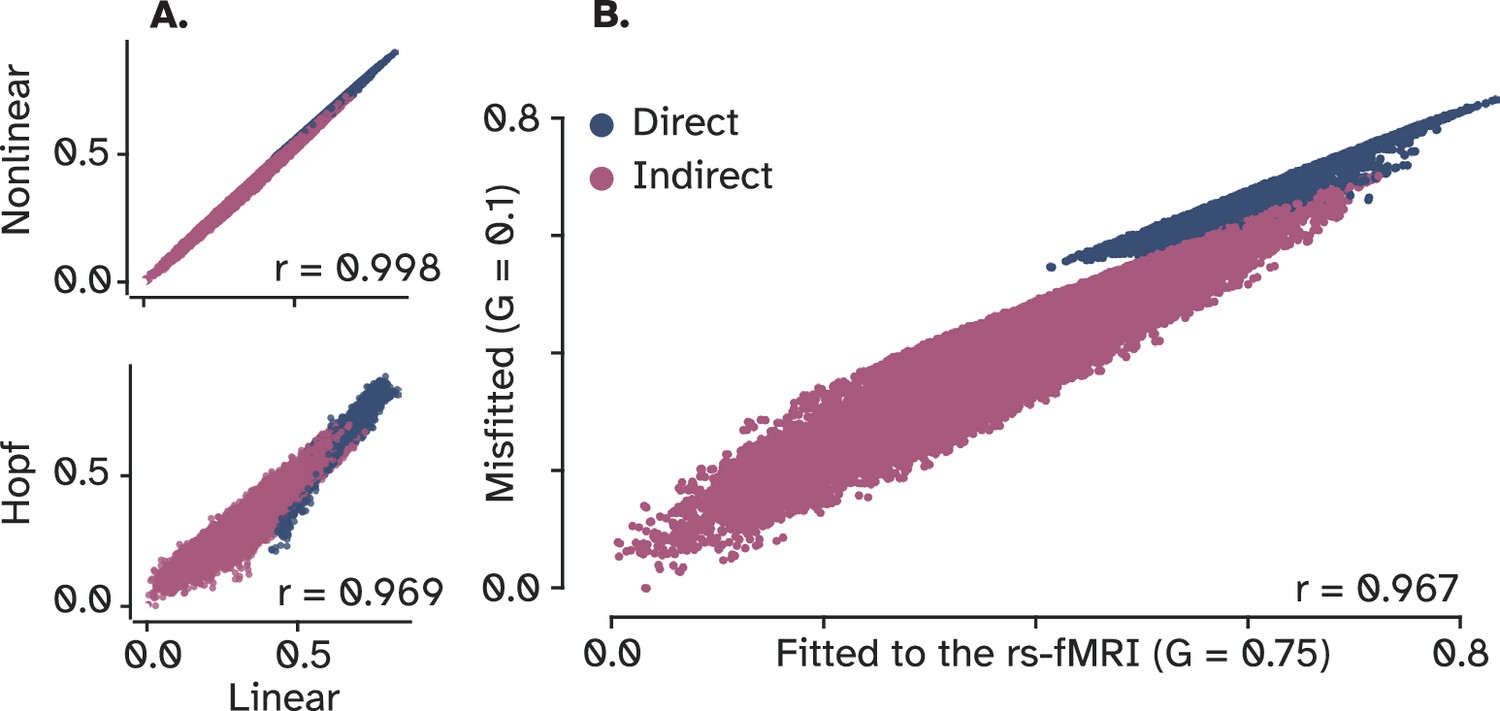
Correlations among linear, nonlinear, and neural mass models of local dynamics.

(A) OI matrices for a linear and a nonlinear model show a near-perfect correlation. Moreover, a Hopf model also has a strong correlation with the linear model, indicating that a linear model of local dynamics represents the communication in brain networks under optimal influence (OI) as well as more complex node models (B) Scatter plot between two settings of the same linear model, one fitted to resting-state fMRI and the other using a random value for the global coupling parameter. The finding provides evidence for the greater role of network’s structure compared to nodal dynamics in shaping brain-wide optimal influence.

Figure 7—figure supplement 1

Download asset Open asset

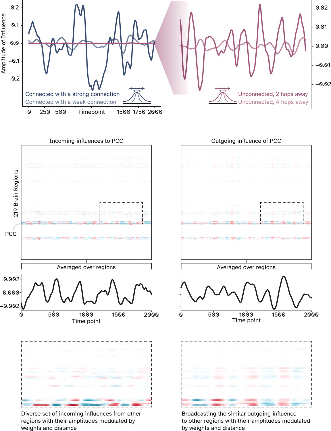
Temporal characteristics of optimal influence, given the Hopf model.

The part above shows how the amplitude of influence between two regions relates to the structural weight and the topological distance between them. The heatmaps in the middle represent the brain-wide incoming and outgoing influence on and from the posterior cingulate cortex (PCC). Together with the column-averaged time course of these influences, the middle plot suggests that PCC receives a diverse range of incoming influences but broadcasts the same message to the rest of the network. This is also apparent from the zoomed-in view of the heatmap at the bottom.

Figure 8 with 2 supplements

Download asset Open asset

Hubs, rich-club nodes, and their influence.

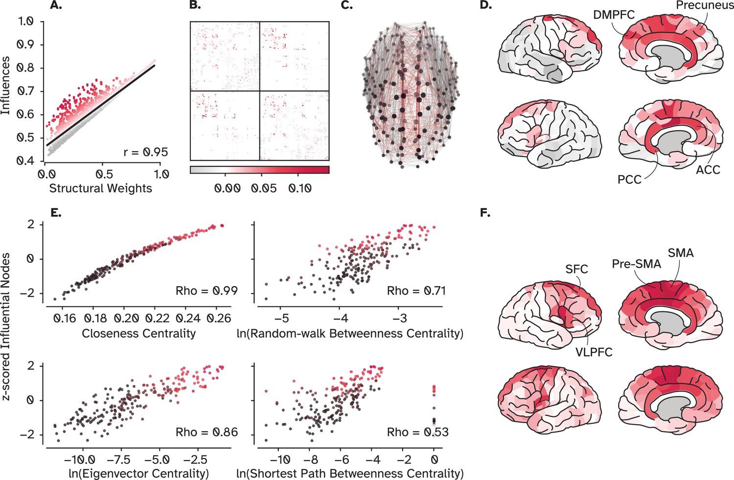
(A) Scatter plot of the influences of nodes on their connected neighbors (direct influence in Figure 2) versus the strength of the underlying connections. Despite the overall strong correlation between the total influence and the strength of structural connections, residuals (depicted by warm colors) reveal several weak connections with more influence than expected by their connection weights. (B) The position of weak connections with strong influence in the adjacency matrix. (C) The position of these connections in the structural brain network shows that they are mainly long-range connections among the hub regions of the cortex. (D) shows those hub regions. (E) The relationship between the influence of a region and its centrality, by four centrality measures (see Material and Methods, Graph-theoretical Measures). (F) The most indirectly influential nodes (indicated by red points in E) that can propagate information to distant and unconnected regions. DMPFC: Dorsomedial prefrontal cortex, PCC: Posterior cingulate cortex, ACC: Anterior cingulate cortex, SFC: Superior frontal cortex, SMA: Supplementary motor area, VLPFC: Ventrolateral prefrontal cortex.

Figure 8—figure supplement 1

Download asset Open asset

The relationship between the log-normalized structural weights and the fiber length, which had a correlation of –0.6, suggesting that the longer the fiber, the weaker its strength is.

Figure 8—figure supplement 2

Download asset Open asset

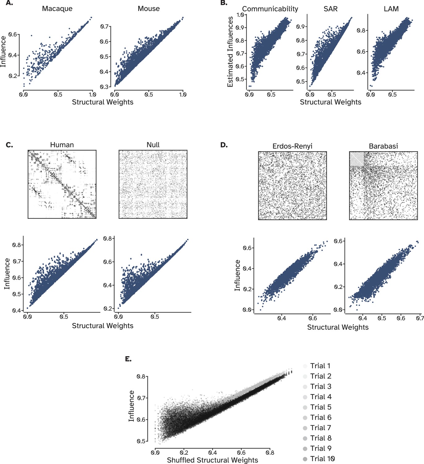
Further analysis of the influence of weak connections in null, synthetic, and supplementary networks.

(A) The relationship between structural weights and the influence of two connected regions in the mouse and macaque connectome supports the results from the human connectome. There exists many weak connections that exert more influence than expected from their connection weights (the ‘bump’) (B) Communication models capture the bump to different extent. (C) The bump is also apparent in the strength-preserved null model, although localized in weaker connections. (D) Two synthetic networks in which both the weights and the topology is randomized did not replicate the bump. (E) Topology-preserved weight-shuffled networks replicated the bump, however, as with C they are localized to weak connections, suggesting a complementary role for both weight distribution and topological features.

Figure 9 with 1 supplement

Download asset Open asset

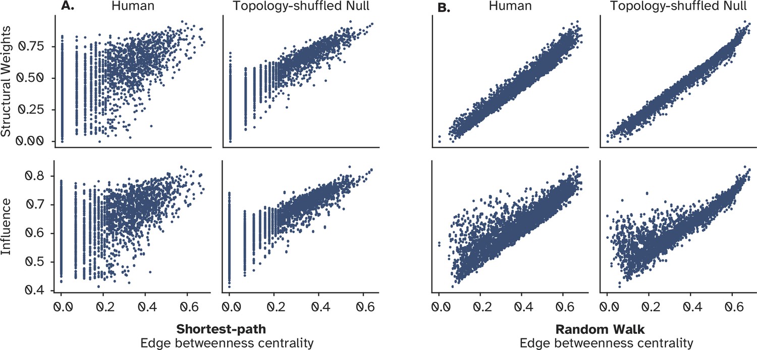
Relationship between the centrality of individual connections and their influence.

(A) Strength of individual connections versus their centrality in terms of shortest-path edge betweenness centrality. The lower panel shows the same relationship, but for the amount of influence a node has over its connected neighbor compared to the centrality of their connections. (B) Depicts the same information for the random walk (diffusive) model of information flow. In both A and B, this relationship is compared against a null model in which the structural connectivity is shuffled while preserving the strength of each node, i.e., the weighted sum of its connections.

Figure 9—figure supplement 1

Download asset Open asset

The relationship between influential nodes (in red) and their controllability measures.

Figure 10

Download asset Open asset

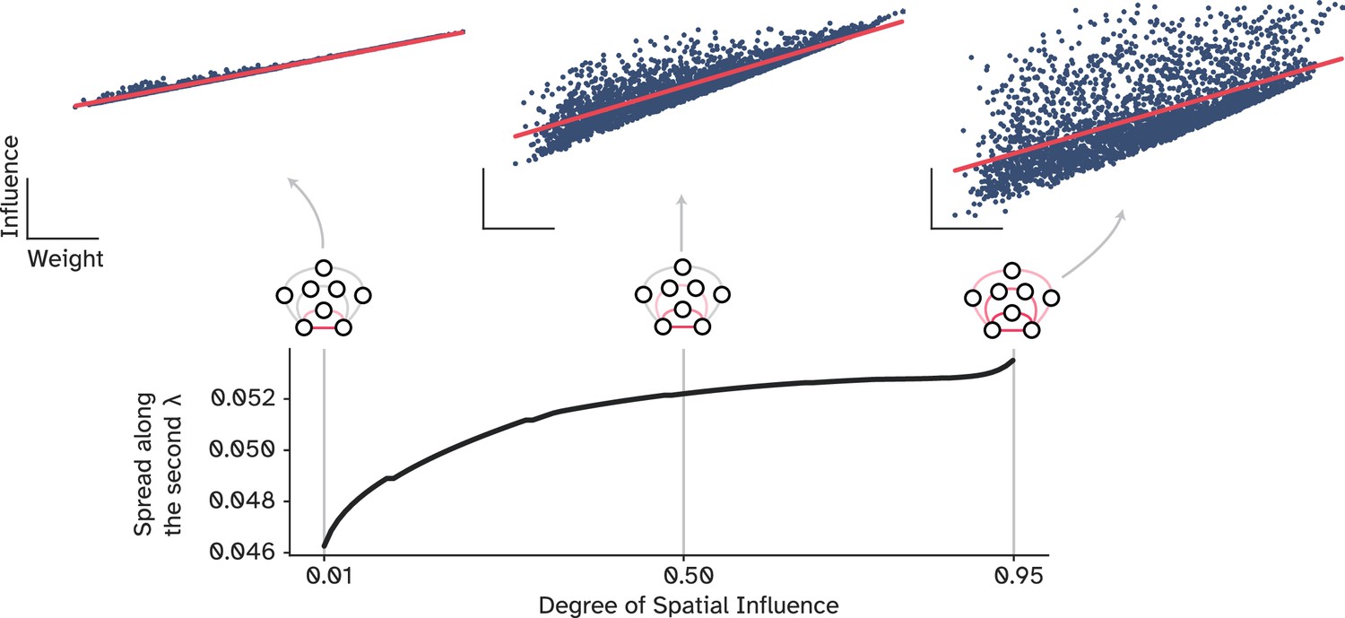
How influence decouples from the underlying structural connections.

The spread of points along the second principal component, i.e., orthogonal to the regression line, across different values of spatial influence. A very small degree of spatial influence represents a case in which the signal can only reach the neighboring nodes, while higher values indicate influences that extend over longer pathways and reverberate in the network, effectively decoupled from the underlying structural weight.

Tables

Table 1

Communication models and measures.

Models	Measures^*	References
Shortest Path Efficiency Floyd-Warshall algorithm	$\begin{array}{ll} S P E & = \frac{1}{Λ^{}} \\ Λ_{i j}^{Ω^{}} & = L_{i u_{1}} + \dots + L_{u_{k} j} \\ Ω_{i j}^{*} & = min_{Ω i j = {i, u_{1}, \dots, u_{k}, j}} \frac{1}{Σ_{l = 1}^{k} w_{u_{l} u_{l + 1}}} \end{array}$	Latora and Marchiori, 2001; Seguin et al., 2020
Navigation Efficiency	$\begin{aligned} N E & = \frac{1}{Λ} \\ Λ_{i j}^{Ω} & = L_{i u_{1}} + \dots + L_{u_{k} j} \\ L_{s t} & = min_{(s, s + 1) \in V} ‖ D_{s t} ‖_{2}^{2} \end{aligned}$	Seguin et al., 2020; Seguin et al., 2018
Diffusion Efficiency	$\begin{array}{ll} D E & = \frac{Σ_{i} Σ_{j} \frac{1}{t_{i j}}}{N (N - 1)}, i \neq j \\ t_{i j} & = \frac{z_{j j} - z_{i j}}{ω_{j}}, i \neq j \\ Z & = [z_{i j}] = (I - \hat{W} + \hat{ω})^{- 1} \\ \hat{W} & = [{\hat{w}}_{i j}], {\hat{w}}_{i j} = \frac{W_{i j}}{Σ_{u = 1}^{N} W_{i u}} \\ ω & = [ω_{1}, \dots, ω_{N}]^{T}, ω {\hat{W}}^{T} = λ ω . \\ \hat{ω} & = [ω, \dots, ω] \end{array}$	Goñi et al., 2013; Seguin et al., 2020
Search Information	$\begin{array}{ll} S I & = - \log_{2} (Π) \\ Π_{Ω_{i j}} & = {\hat{w}}_{i u} \times \dots \times {\hat{w}}_{i j} \end{array}$	Seguin et al., 2019; Seguin et al., 2020
Communicability	$\begin{aligned} C O & = [c o_{i j}] \\ c o_{i j} & = Σ_{k = 0}^{\infty} \frac{(\hat{W})_{i j}^{k}}{k!} = e^{\hat{W}} \end{aligned}$	Chen et al., 2022b; Estrada and Hatano, 2008
Scaled Communicability	$\begin{aligned} S C O & = [s c o_{i j}] \\ s c o_{i j} & = Σ_{k = 0}^{\infty} \frac{(α \hat{W})_{i j}^{k}}{k!} = e^{α \hat{W}} \end{aligned}$	Ghosh et al., 2023; Messé et al., 2014
Linear Attenuation	$\begin{aligned} L A M & = (I - α \hat{W})^{- 1} \end{aligned}$	Goñi et al., 2013
Spatial Autoregressive	$\begin{aligned} S A R & = (I - α \hat{W})^{- 1} (I - α \hat{W})^{- T} \end{aligned}$	Zamora-López et al., 2016

*

Throughout the table, $W \in R^{N \times N}$ is the adjacency matrix corresponding to a given graph, $G = (V, E)$ with $N$ vertices (nodes). $W_{i j}$ signifies the connection strength from vertex i to vertex j. Anatomical connections are indicated by $W_{i j} > 0$ for connected region pairs and $W_{i j} = 0$ for unconnected pairs. $L$ denotes the matrix of path lengths, defined as the reciprocal of $W$ , such that $L = \frac{1}{W}$ with $L_{i j}$ as the path length between two connected nodes, i and j. Further, $Ω_{i j} = {u_{1}, u_{2}, \dots, u_{k}}$ is the sequence of nodes visited along the shortest path between nodes i and j. Given the spatial organization of nodes in empirical structural connectivity, $D_{s t}$ includes the Euclidean distance between source, s, and destination, t nodes in finding optimal paths. The term $\hat{W}$ signifies the normalized adjacency matrix, where each element ${\hat{w}}_{i j}$ is obtained by dividing the original connection strength, $w_{i j}$ by the sum of all connection strengths in the corresponding row of the matrix $W$ . $I$ is the identity matrix, $T$ stands for transposed inverse matrix, and $α < \frac{1}{λ_{m a x}}$ where $λ_{m a x}$ is the spectral radius of the adjacency matrix, $W$ . $λ$ denotes the eigenvalues of a given matrix.

Table 2

Graph-theoretical measures.

Types	Measures^*	References
Closeness Centrality	$C_{C} (i) = \frac{N - 1}{Σ_{j = 1, j \neq i}^{N} d_{i j}}$	Oldham et al., 2019
Eigenvector Centrality	$C_{E} (i) = \| v_{i} \|, W v = λ v$	Oldham et al., 2019
Node Betweenness Centrality	$C_{B} (i) = Σ_{s \neq i \neq t} \frac{σ_{s t} (i)}{σ_{s t}}$	Oldham et al., 2019; Zuo et al., 2012
Edge Betweenness Centrality	$C_{B_{e d g e}} (e) = Σ_{s \neq t} \frac{σ_{s t} (e)}{σ_{s t}}$	Oldham et al., 2019; Zuo et al., 2012
Random Walk Centrality	$\begin{aligned} T & = D - A, D_{i i} = Σ_{j = 1}^{N} W_{i j} \\ V_{s t}^{i} & = T_{i s} - T_{i t} \\ I_{s t}^{i} & = \frac{1}{2} Σ_{j} W_{i j} \| V_{s t}^{i} - V_{s t}^{j} \| \\ C_{R W} (i) & = \frac{Σ_{s < t} I_{s t}^{i}}{\frac{1}{2} N (N - 1)} \end{aligned}$	Newman, 2005
Average Controllability	$\begin{aligned} W & = U^{*} T U \\ M & = (U \circ U)^{T} \\ v & = d i a g (T) \\ P & = d i a g (1 - v v^{T}) \\ P & = [P_{diag}, \dots, P_{diag}] \\ C_{a v g} & = \sum (\frac{M}{P}) \end{aligned}$	Gu et al., 2015
Modal Controllability	$\begin{aligned} W & = U^{*} T U \\ v & = [v_{1}, \dots, v_{N}] = d i a g (T) \\ C_{M} (i) & = Σ_{j = 1}^{N} U_{i j}^{2} (1 - v_{j}^{2}) \end{aligned}$	Gu et al., 2015

*

Throughout the table, $W ϵ R^{N \times N}$ is the adjacency matrix corresponding to a given graph, $G = (V, E)$ with vertices (nodes) $W_{i j}$ signifies the connection strength from vertex i to vertex j Anatomical connections are indicated by $W_{i j} > 0$ for connected region pairs and for $W_{i j} = 0$ unconnected pairs. $d_{s t}$ denotes the shortest path distance between s nodes and, t and $σ_{s t}$ is the total number of shortest paths from node s to node t and $σ_{s t} (i)$ is the number of those paths that pass through node i.In edge betweenness centrality, $σ_{s t} (e)$ stands for the number of those paths that pass through a given edge, e. Further, v refers to the left eigenvector associated with the eigenvalue of λ maximum modulus. In computing controllability measures, we used Schur decomposition to find the unitary matrix, $U$ , and the upper triangular matrix, $T$ , to express the adjacency matrix, $W$ . Further, $\circ$ denotes element-wise multiplication, * represents the conjugate transpose, and $d i a g (.)$ extracts the diagonal elements.

Additional files

MDAR checklist: https://cdn.elifesciences.org/articles/101780/elife-101780-mdarchecklist1-v1.docx
Download elife-101780-mdarchecklist1-v1.docx

Download links

A two-part list of links to download the article, or parts of the article, in various formats.

Downloads (link to download the article as PDF)

Open citations (links to open the citations from this article in various online reference manager services)

Mendeley

Cite this article (links to download the citations from this article in formats compatible with various reference manager tools)

Kayson Fakhar
Fatemeh Hadaeghi
Caio Seguin
Shrey Dixit
Arnaud Messé
Gorka Zamora-López
Bratislav Misic
Claus C Hilgetag

(2025)

A general framework for characterizing optimal communication in brain networks

eLife 13:RP101780.

https://doi.org/10.7554/eLife.101780.3

Share this article

Cite this article

Overview of the present work.

Visual summary of the multi-perturbation Shapley value analysis (MSA) approach.

Comparing the optimal influence matrices from 1000 and 10,000 lesion samples per source node.

Large-scale network organization of the optimal influence landscape.

Comparison of optimal influences with other putative communication measures.

Comparing optimal influence with functional connectivity.

Strategies to alleviate the underestimated influence of long-range pathways.

Fitting curve of the scaled communicability (left) and the linear attenuation model (right) to the optimal influence matrix of the human connectome.

Fitting curves of the spatial autoregressive model (top), scaled communicability (middle) and the linear attenuation model (bottom) to the optimal influence matrix of macaque (left) and mouse (right) connectomes.

Uni-and-multivariate models of OI.

The amount of which univariate and multivariate models can predict optimal influence from summing individual walks, discounted exponentially (as with communicability).

Correlations among linear, nonlinear, and neural mass models of local dynamics.

Temporal characteristics of optimal influence, given the Hopf model.

Hubs, rich-club nodes, and their influence.

The relationship between the log-normalized structural weights and the fiber length, which had a correlation of –0.6, suggesting that the longer the fiber, the weaker its strength is.

Further analysis of the influence of weak connections in null, synthetic, and supplementary networks.

Relationship between the centrality of individual connections and their influence.

The relationship between influential nodes (in red) and their controllability measures.

How influence decouples from the underlying structural connections.

Communication models and measures.

Graph-theoretical measures.

MDAR checklist

Downloads (link to download the article as PDF)

Open citations (links to open the citations from this article in various online reference manager services)

Cite this article (links to download the citations from this article in formats compatible with various reference manager tools)