Q-learning with temporal memory to navigate turbulence
- MaLGa, Department of Computer Science, Bioengineering, Robotics and Systems Engineering, University of Genova, Italy
- MalGa, Department of Civil, Chemical and Environmental Engineering, University of Genoa, Italy
Figures
Figure 1
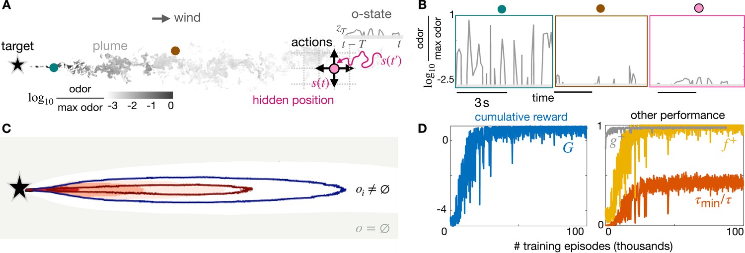
Learning a stimulus-response strategy for turbulent navigation.
(A) Representation of the search problem with turbulent odor cues obtained from Direct Numerical Simulations of fluid turbulence (gray scale, odor snapshot from the simulations). The discrete position is hidden; the odor concentration is observed along the trajectory , where is the sensing memory. (B) Odor traces from direct numerical simulations at different (fixed) points within the plume. Odor is noisy and sparse, information about the source is hidden in the temporal dynamics. (C) Contour maps of olfactory states with nearly infinite memory (): on average, olfactory states map to different locations within the plume, and the void state is outside the plume. Intermittency is discretized in three bins defined by two thresholds: 66% (red line) and 33% (blue line). Intensity is discretized in 5 bins (dark red shade to white shade) defined by four thresholds (percentiles 99%, 80%, 50%, 25%). (D) Performance of stimulus-response strategies obtained during training, averaged over 500 episodes. We train using realistic turbulent data with memory and backtracking recovery.
Figure 2 with 1 supplement
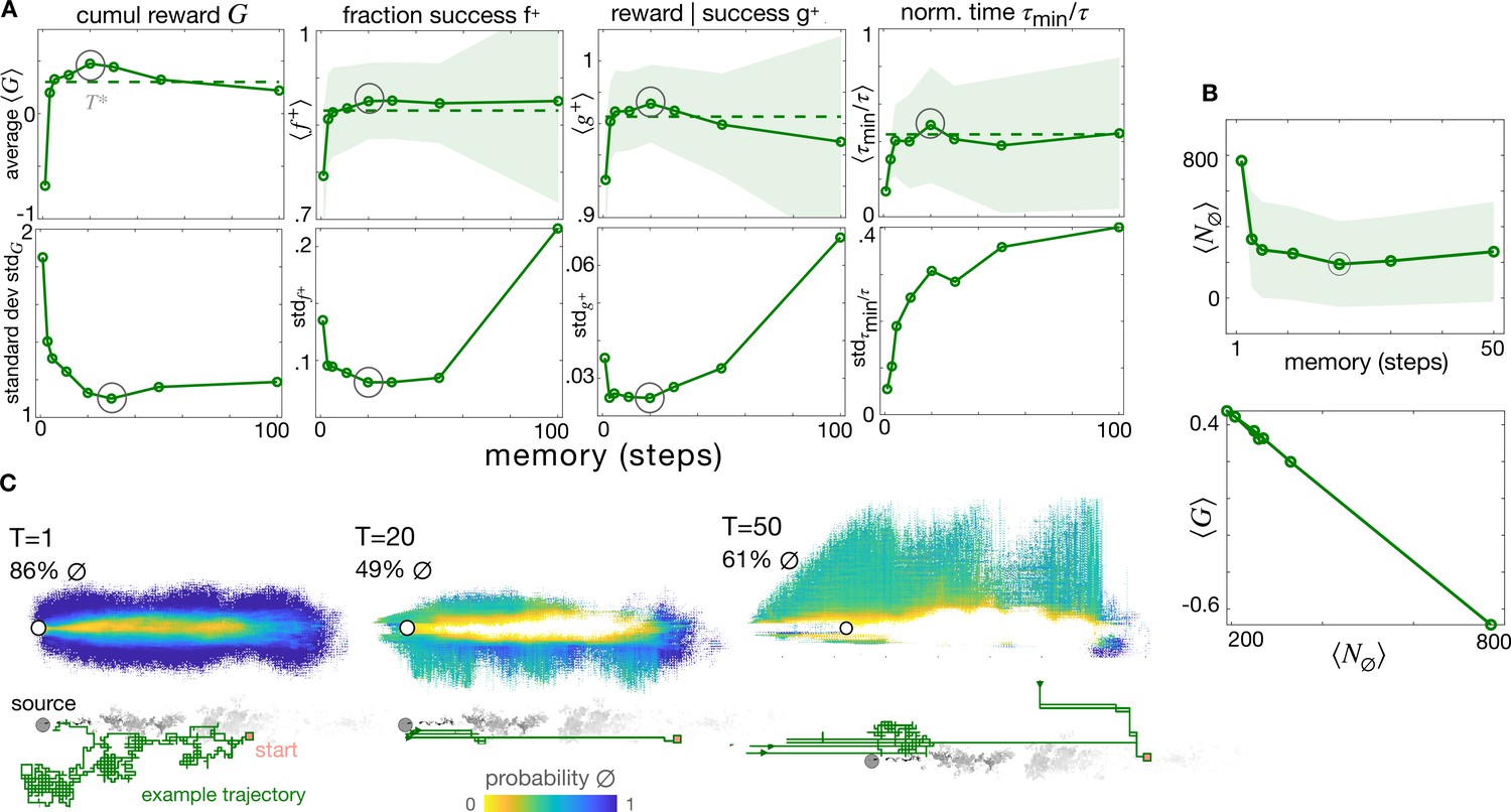
The optimal memory .
(A) Four measures of performance as a function of memory with backtracking recovery (solid line) show that the optimal memory maximizes average performance and minimizes standard deviation, except for the normalized time. Top: Averages computed over 10 realizations of test trajectories starting from 43,000 initial positions (dash: results with adaptive memory). Bottom: standard deviation of the mean performance metrics for each initial condition (see Materials and methods). (B) Average number of times agents encounter the void state along their path, , as a function of memory (top); cumulative average reward is inversely correlated to (bottom), hence the optimal memory minimizes encounters with the void. (C) Colormaps: Probability that agents at different spatial locations are in the void state at any point in time, starting the search from anywhere in the plume and representative trajectory of a successful searcher (green solid line) with memory , , (left to right). At the optimal memory, agents in the void state are concentrated near the edge of the plume. Agents with shorter memories encounter voids throughout the plume; agents with longer memories encounter more voids outside of the plume as they delay recovery. In all panels, shades are ± standard deviation.
Figure 2—figure supplement 1
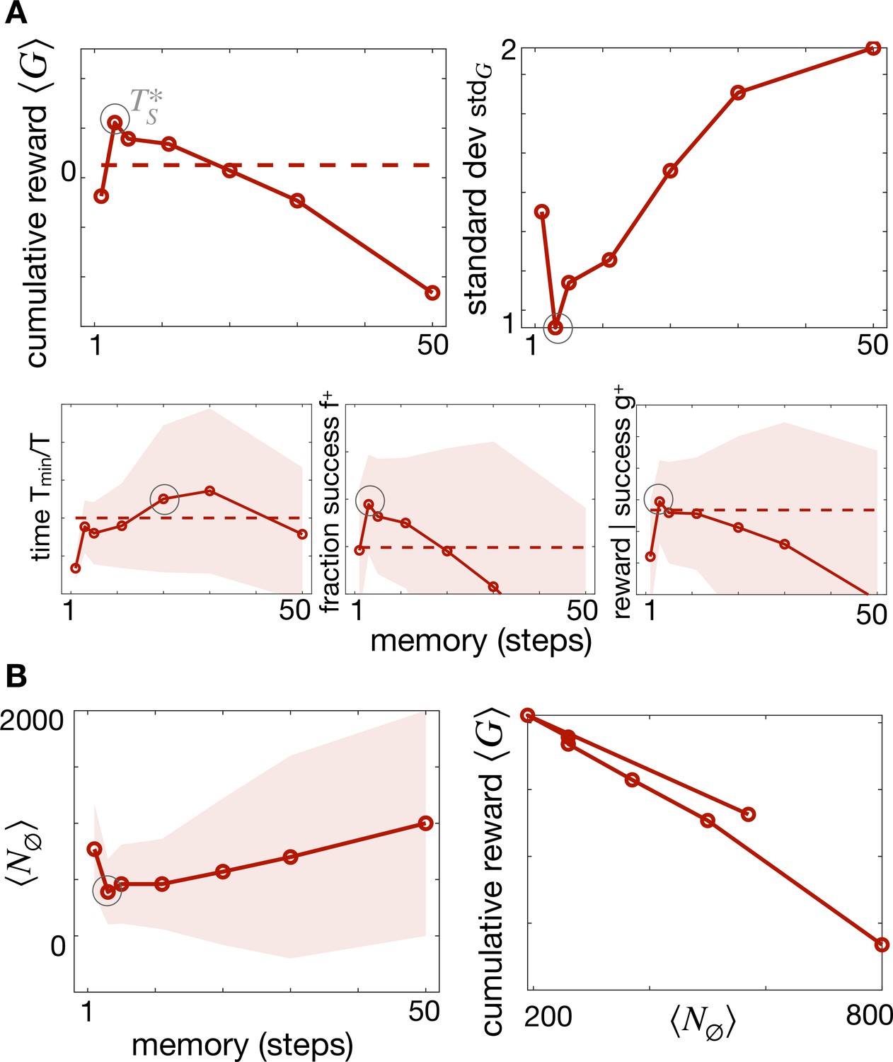
The role of temporal memory with Brownian recovery strategy (same as main Figure 2A).
(A) Total cumulative reward (top left) and standard deviation (top right) as a function of memory showing an optimal memory for the Brownian agent. Other measures of performance with their standard deviations show the same optimal memory (bottom). The trade-off between long and short memories discussed in the main text holds, but here exiting the plume is much more detrimental because regaining position within the plume by Brownian motion is much lengthier. (B) As for the Backtracking agent, the optimal memory corresponds to minimizing the number of times the agent encounters the void state.
Figure 3 with 1 supplement
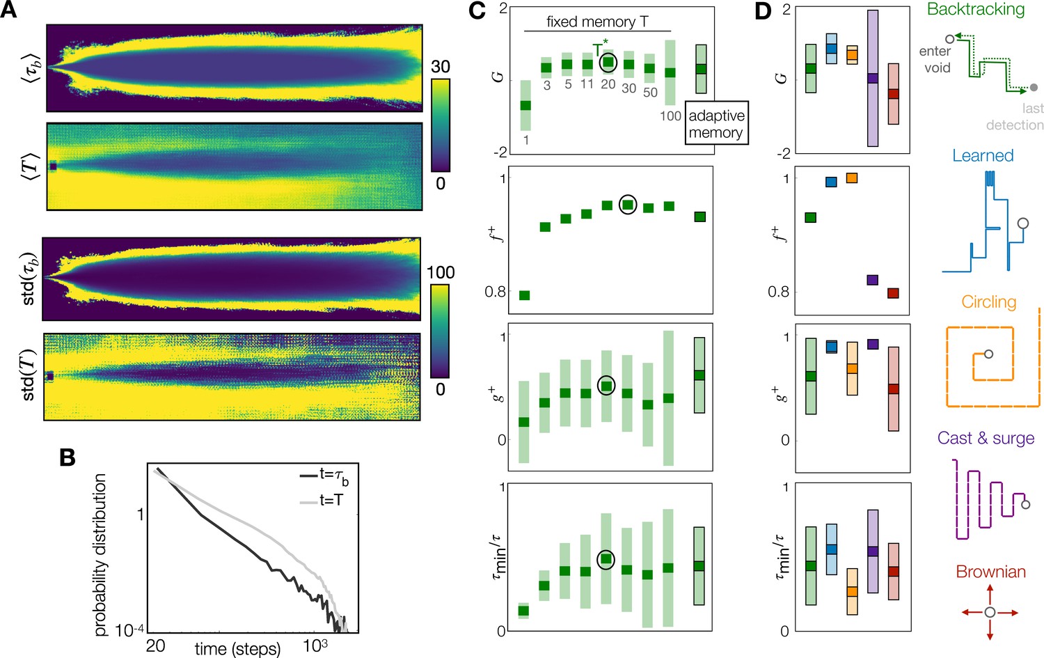
The adaptive memory approximates the duration of the blank dictated by physics, and it is an efficient heuristic, especially when coupled with a learned recovery strategy.
(A) Top to bottom: Colormaps of the Eulerian average blank time ; average sensing memory ; standard deviation of Eulerian blank time and of sensing memory. The sensing memory statistics are computed over all agents that are located at each discrete cell, at any point in time. (B) Probability distribution of across all spatial locations and times (black) and of across all agents at all times (gray). (C) Performance with the adaptive memory nears performance of the optimal fixed memory, here shown for backtracking; similar results apply to the Brownian recovery (Figure 3—figure supplement 1). (D) Comparison of five recovery strategies with adaptive memory: The learned recovery with adaptive memory outperforms all fixed and adaptive memory agents. In (C) and (D), dark squares mark the mean, and light rectangles mark ± standard deviation. is defined as the fraction of agents that reach the target at test, hence has no standard deviation.
Figure 3—figure supplement 1
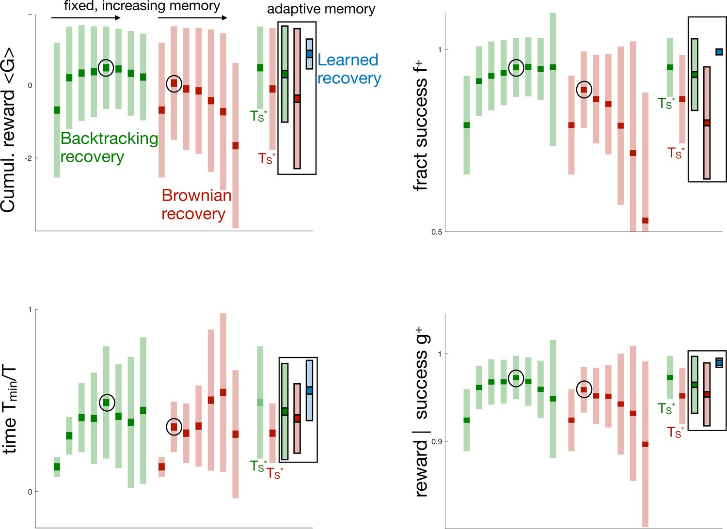
All four measures of performance across agents with fixed memory and Backtracking vs Brownian recovery (green and red respectively, unframed boxes) and with adaptive memory for Backtracking, Brownian, and Learned recovery (green, red, and blue respectively, framed boxes).
Figure 4 with 2 supplements
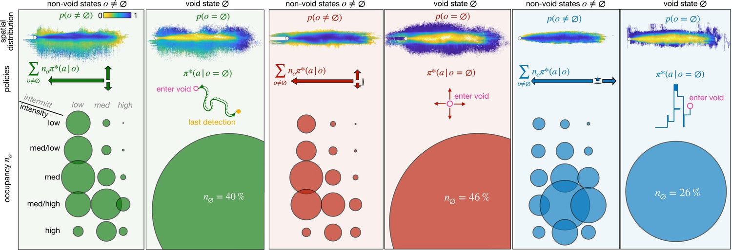
Optimal policies with adaptive memory for different recovery strategies: backtracking (green), Brownian (red), and learned (blue).
For each recovery, we show the spatial distribution of the olfactory states (top); the policy (center) and the state occupancy (bottom) for non-void states (left) vs the void state (right). Spatial distribution: probability that an agent at a given position is in any non-void olfactory state (left) or in the void state (right), color-coded from yellow to blue. Policy: actions learned in the non-void states , weighted on their occupancy (left, arrows proportional to the frequency of the corresponding action) and schematic view of recovery policy in the void state (right). State occupancy: fraction of agents that is in any of the 15 non-void states (left) or in the void state (right) at any point in space and time. Occupancy is proportional to the radius of the corresponding circle. The position of the circle identifies the olfactory state (rows and columns indicate the discrete intensity and intermittency respectively). All statistics are computed over 43,000 trajectories, starting from any location within the plume.
Figure 4—figure supplement 1
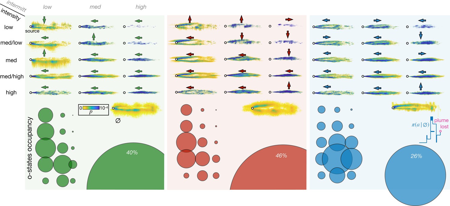
Optimal policies for different recovery strategies and adaptive memory.
From left to right: results for backtracking (green), Brownian (red), and learned (blue) recovery strategies. Top: probability that an agent in a given olfactory state is at a specific spatial location color-coded from yellow to blue. Rows and columns indicate the olfactory state; the void state is in the lower right corner. Arrows indicate the optimal action from that state. Bottom: Circles represent occupancy of each state, olfactory states are arranged as in the top panel. All statistics are computed over 43,000 trajectories, starting from any location within the plume.
Figure 4—figure supplement 2
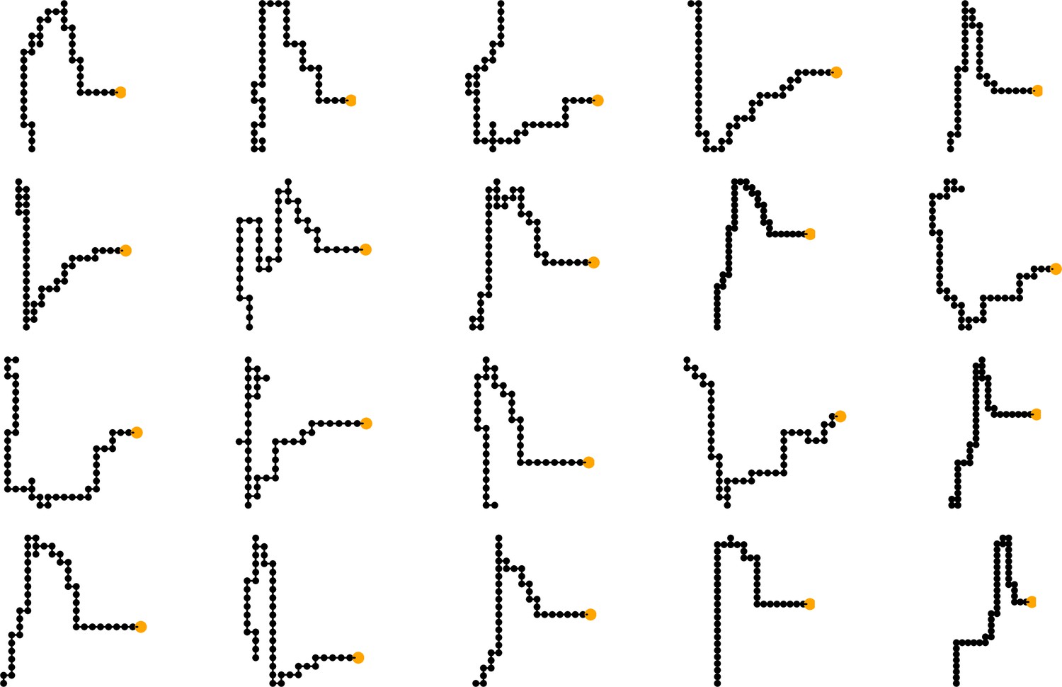
The learned recovery resembles the cast and surge observed in animals, with an initial surge of 5±2 steps and a subsequent motion crosswind starting from either side of the centerline and overshooting to the other side.
Figure 5 with 1 supplement
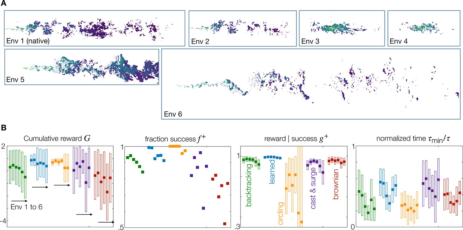
Generalization to statistically different environments.
(A) Snapshots of odor concentration normalized with concentration at the source, color-coded from blue (0) to yellow (1) for environment 1–6 as labeled. Environment 1 is the native environment where all agents are trained. (B) Performance for the five recovery strategies backtracking (green), learned (blue), circling (orange), zigzag (purple) and brownian (red), with adaptive memory, trained on the native environment and tested across all environments 1–6. Four measures of performance defined in the main text are shown. Dark squares mark the mean, and empty rectangles ± standard deviation. For definition of the metrics used, see Materials and Methods, Agents Evaluation.
Figure 5—figure supplement 1
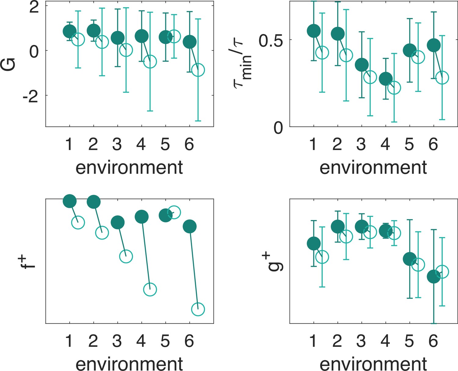
The learned recovery with adaptive memory and a single non-empty olfactory state (empty circles) displays degraded performance with respect to the full model (full circles).
Tables
Table 1
Parameters of the learned recovery, statistics over 20 independent trainings.
| Initial surge upwind | 6 ± 2 |
|---|---|
| Total steps upwind | 15 ± 2 |
| Total steps downwind | 1.3 ± 1.4 |
| Total steps to the right | 15 ± 3 |
| Total steps to the left | 18 ± 6 |
Key resources table
| Reagent type (species) or resource | Designation | Source or reference | Identifiers | Additional information |
|---|---|---|---|---|
| Software, algorithm | Computational fluid dynamics source code | Viola et al., 2023; Viola et al., 2020; Viola et al., 2022; Verzicco et al., 2025. Courtesy of F. Viola. | https://gitlab.com/vdv9265847/IBbookVdV/ | Reused Computational Fluid Dynamics software used to run simulations of odor transport. An earlier version of the code is publicly available at the website indicated in the ‘identifiers’ entry, described in Verzicco et al., 2025. Our simulations were conducted using a GPU-accelerated version of the code that was developed by F. Viola and colleagues in the Refs indicated in the ‘Source or reference’ entry. This version will be shared in the near future. All requests may be directed to Viola and colleagues |
| Software, algorithm | Datasets of odor field obtained with computational fluid dynamics – Environments 5 and 6 | This paper | https://doi.org/10.5281/zenodo.14655991 | Newly developed datasets of turbulent odor fields, obtained through computational fluid dynamics. |
| Software, algorithm | Tabular Q-learning | This paper, Rando, 2025 | https://github.com/Akatsuki96/qlearning_for_navigation | Newly developed Model-free Algorithm for training olfactory search agents, with settings described in materials and methods. Shared on github address mentioned as ‘Identifier’ |
| Software, algorithm | Datasets of odor field obtained with computational fluid dynamics – Environments 1–4 | Rigolli et al., 2022b | https://doi.org/10.5281/zenodo.6538177 | Reused datasets of turbulent odor fields, obtained through computational fluid dynamics in Rigolli et al., 2022b |
Table 2
Gridworld geometry.
From Top: 2D size of the simulation, agents that leave the simulation box continue to receive negative reward and no odor; number of time stamps in the simulation, beyond which simulations are looped; number of actions per time stamp; speed of the agent; noise level below which odor is not detected; location of the source on the grid. See Table 3 for the values of the grid size and time stamps at which odor snapshots are saved.
| Simulation 1 | Simulation 2 | Simulation 3 | |
|---|---|---|---|
| 2D simulation grid | 1225 × 280 | 1024 × 256 | 2000 × 500 |
| # time stamps | 2598 | 5000 | 5000 |
| # decisions per time stamp | 1 | 1 | 1 |
| Speed (grid points / time stamp) | 10 | 10 | 10 |
| Source location | (20, 142) | (128, 128) | (150, 250) |
Table 3
Parameters of the simulations.
From Left to Right: Simulation ID (1, 2, 3); Length , width , height of the computational domain; mean horizontal speed ; Kolmogorov length scale where is the kinematic viscosity and is the energy dissipation rate; mean size of gridcell ; Kolmogorov timescale ; energy dissipation rate ; wall unit where is the friction velocity; bulk Reynolds number based on the bulk speed and half height; magnitude of velocity fluctuations relative to the bulk speed; large eddy turnover time frequency at which odor snapshots are saved . For each simulation, the first row reports results in non-dimensional units. Second and third rows provide an idea of how non-dimensional parameters match dimensional parameters in real flows in air and water, assuming the Kolmogorov length is 1.5 mm in air and 0.4 mm in water.
| Sim ID | |||||||||||||
|---|---|---|---|---|---|---|---|---|---|---|---|---|---|
| 1 | 40 | 8 | 4 | 23 | 0.006 | 0.025 | 0.01 | 39 | 0.0035 | 11500 | 15% | 1 | |
| air | 9.50 m | 1.90 m | 0.96 m | 0.15 cm | 0.6 cm | 0.15 s | 0.09 cm | ||||||
| water | 2.66 m | 0.53 m | 0.27 m | 0.04 cm | 0.2 cm | 0.18 s | 0.02 cm | ||||||
| 2 | 20 | 5 | 2 | 14 | 0.004 | 0.02 | 0.005 | 163 | 0.0038 | 7830 | 15% | 5 | |
| air | 7.50 m | 1.875 m | 0.75 m | 0.15 cm | 0.75 cm | 0.15 s | 0.142 cm | ||||||
| water | 2.00 m | 0.50 m | 0.20 m | 0.04 cm | 0.2 cm | 0.18 s | 0.038 cm | ||||||
| 3 | 20 | 5 | 2 | 22 | 0.0018 | 0.01 | 0.0025 | 204 | 0.0012 | 17500 | 13% | 2.5 | |
| air | 16.7 m | 4.18 m | 1.67 m | 0.15 cm | 0.83 cm | 0.15 s | 0.1 cm | ||||||
| water | 4.44 m | 1.11 m | 0.44 m | 0.04 cm | 0.22 cm | 0.18 s | 0.03 cm |
Additional files
Download links
A two-part list of links to download the article, or parts of the article, in various formats.
Downloads (link to download the article as PDF)
Open citations (links to open the citations from this article in various online reference manager services)
Cite this article (links to download the citations from this article in formats compatible with various reference manager tools)
Q-learning with temporal memory to navigate turbulence
eLife 13:RP102906.
https://doi.org/10.7554/eLife.102906.3


